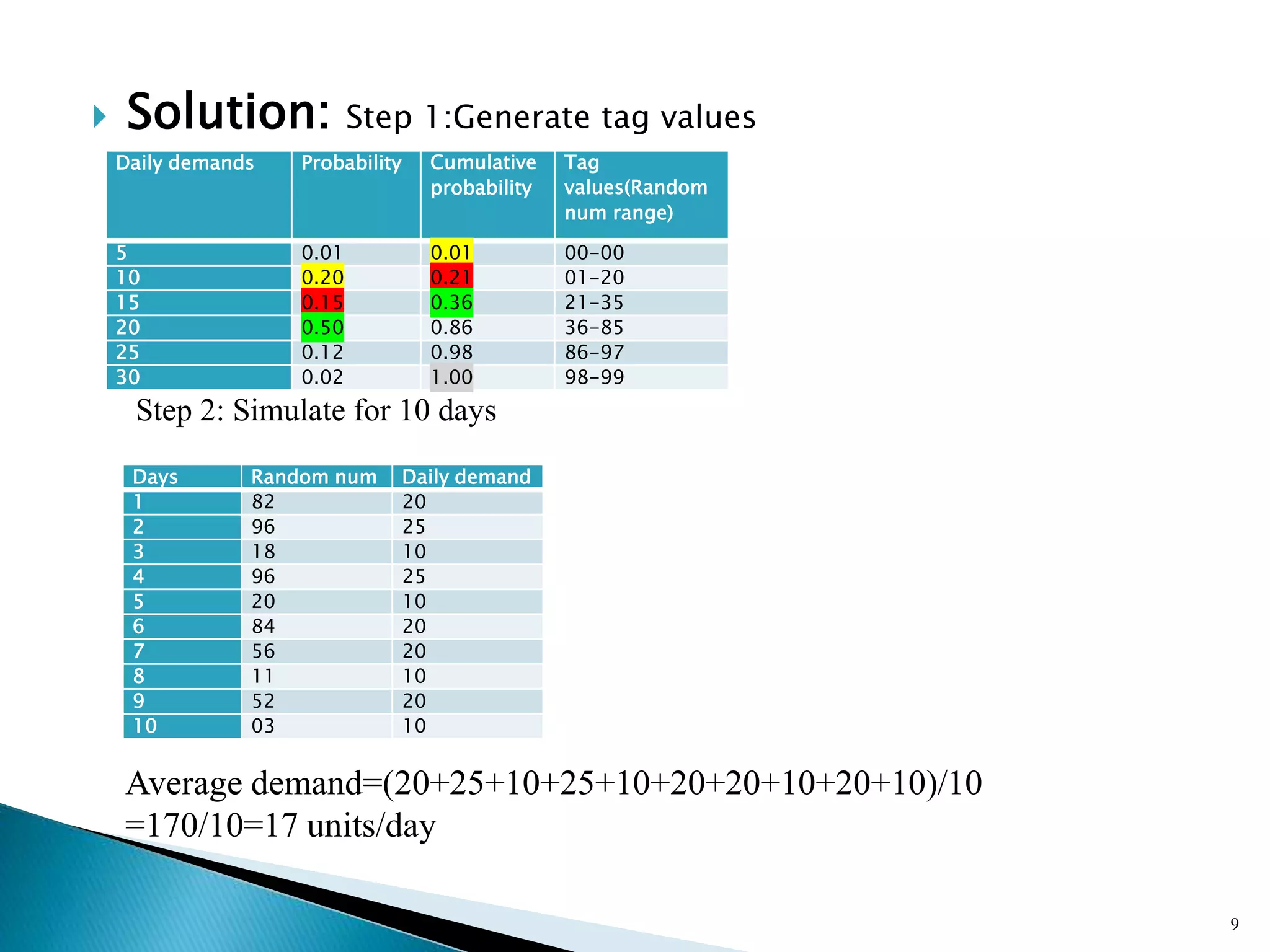
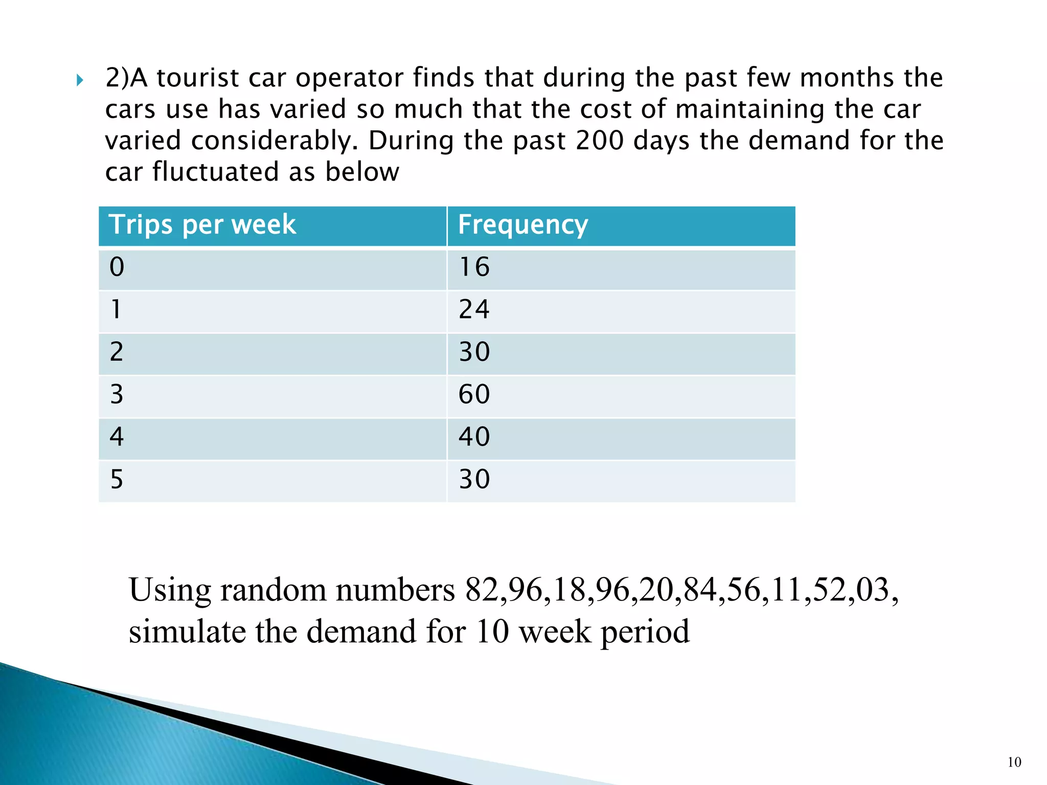
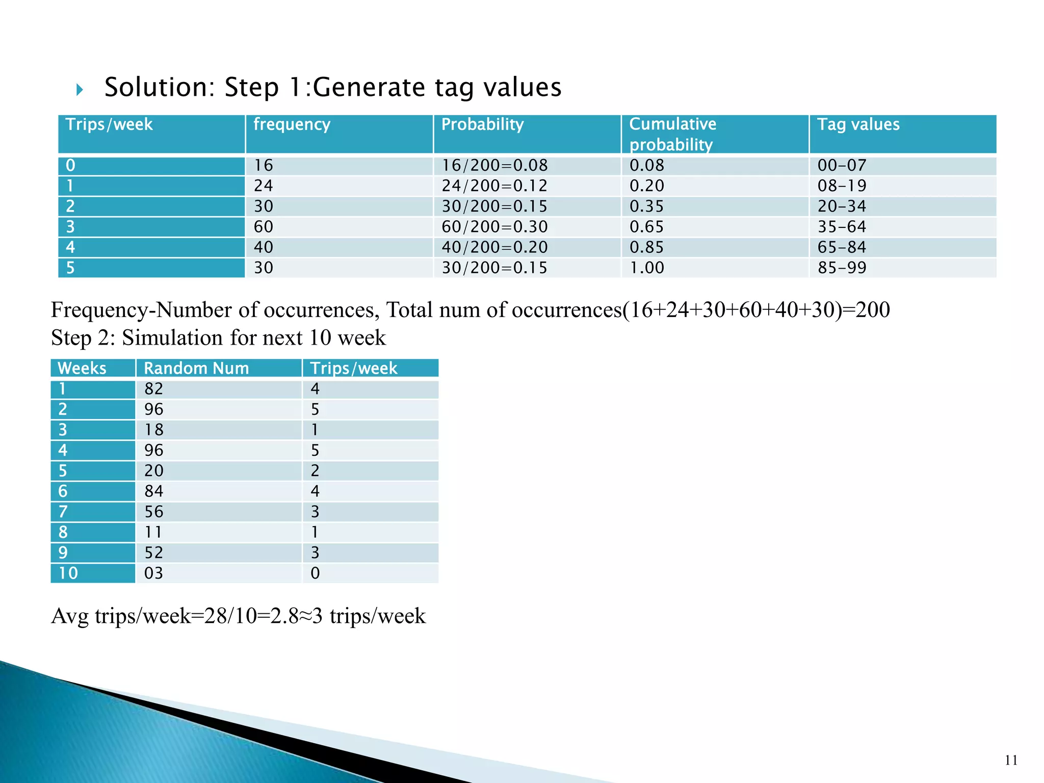
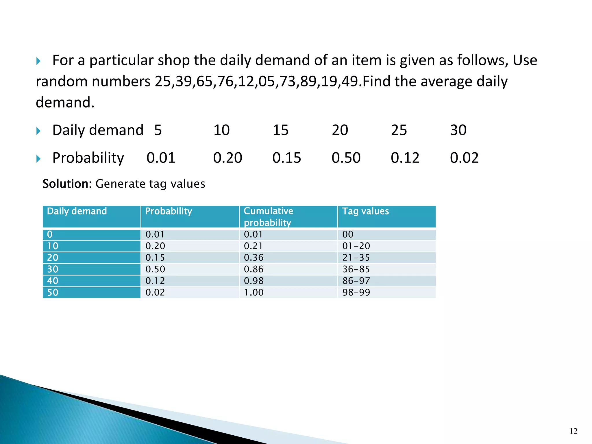
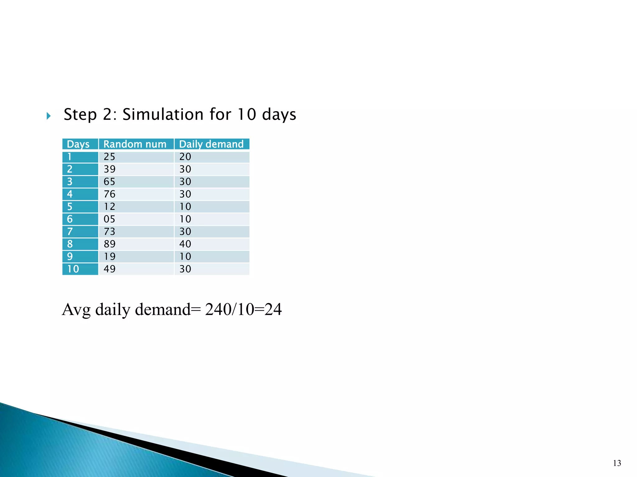
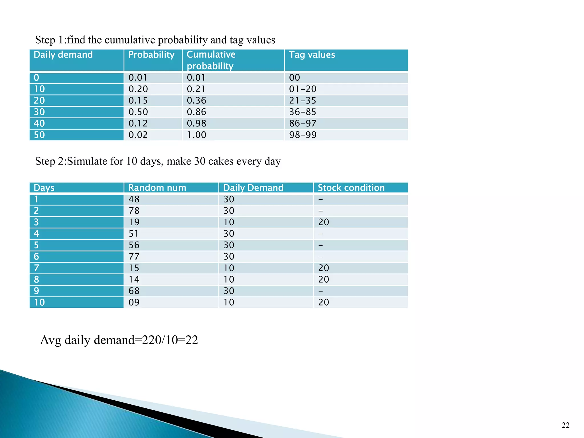
The document describes a Monte Carlo simulation process for modeling uncertainty. It provides examples of simulating daily demand for a bakery and a car rental company using random numbers and probability distributions. For the bakery, the average daily demand over 5 days was calculated to be 17 units. For the car rental company, the average number of trips per week over 10 weeks was calculated to be 2.8 trips. The document demonstrates how Monte Carlo simulation can be used to model systems with uncertain variables and calculate average outcomes.


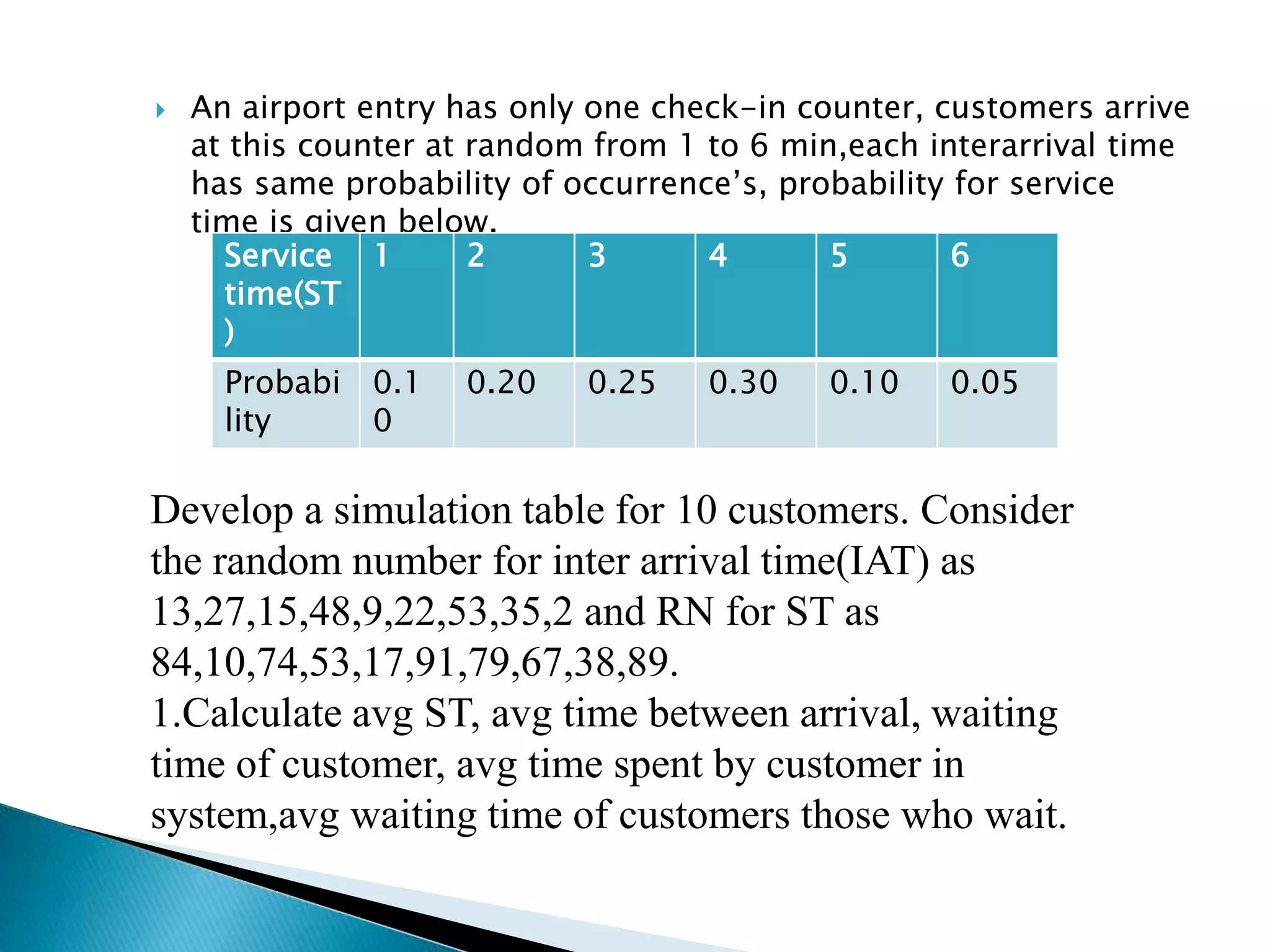
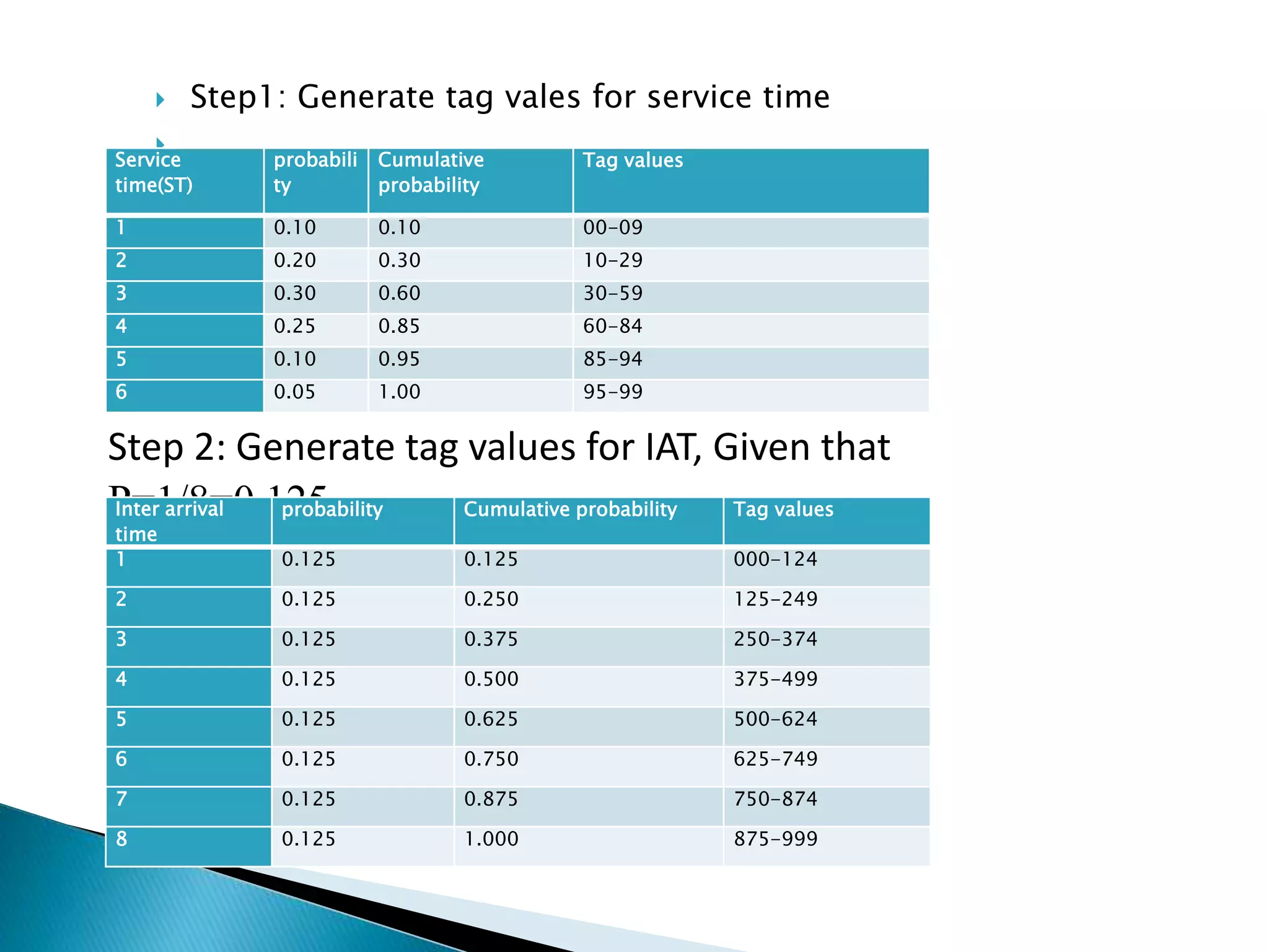
![ step 1:tag values for service time
Service time probability Cumulative
probability
Tag values
1 0.10 0.10 00-09
2 0.20 0.30 10-29
3 0.25 0.55 30-54
4 0.30 0.85 55-84
5 0.10 0.95 85-94
6 0.05 1.00 95-99
Step 2: tag values for IAT, equal probability of occurance[out
of 6 option any one can occur,
1/6=0.166666667=0.17(approx.)]
Inter arrival time probability Cumulative
probability
Tag values
1 1/6=0.17 0.17 00-16
2 0.17 0.34 17-33
3 0.17 0.51 34-50
4 0.17 0.68 51-67
5 0.17 0.85 68-84
6 0.17 1.00 85-99](https://image.slidesharecdn.com/unit4-queuingandsimulation-210522141940/75/Unit-4-simulation-and-queing-theory-m-m-1-24-2048.jpg)