![Gnuplot Script
# Script to plot 1D dataset
reset
unset label
unset key
set key left top
set xrange [0:10]
set yrange [-3:3]
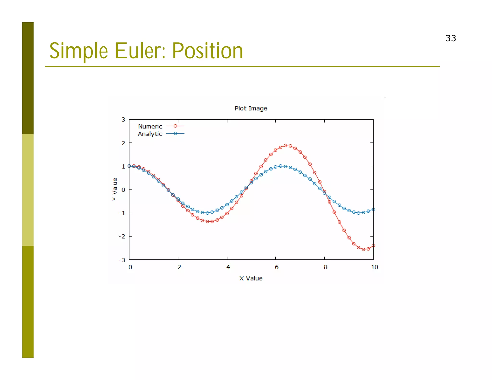
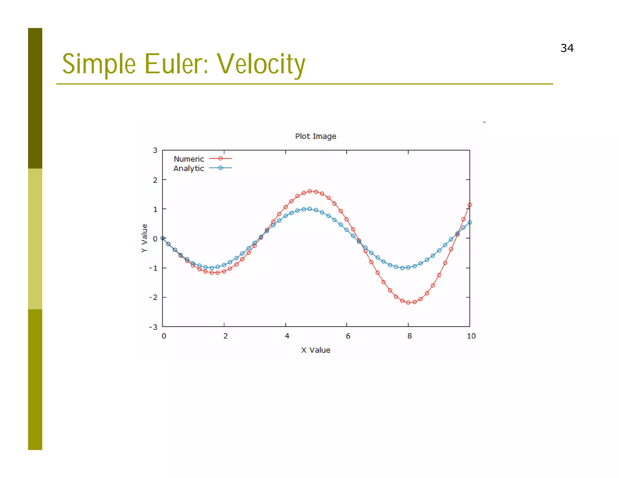
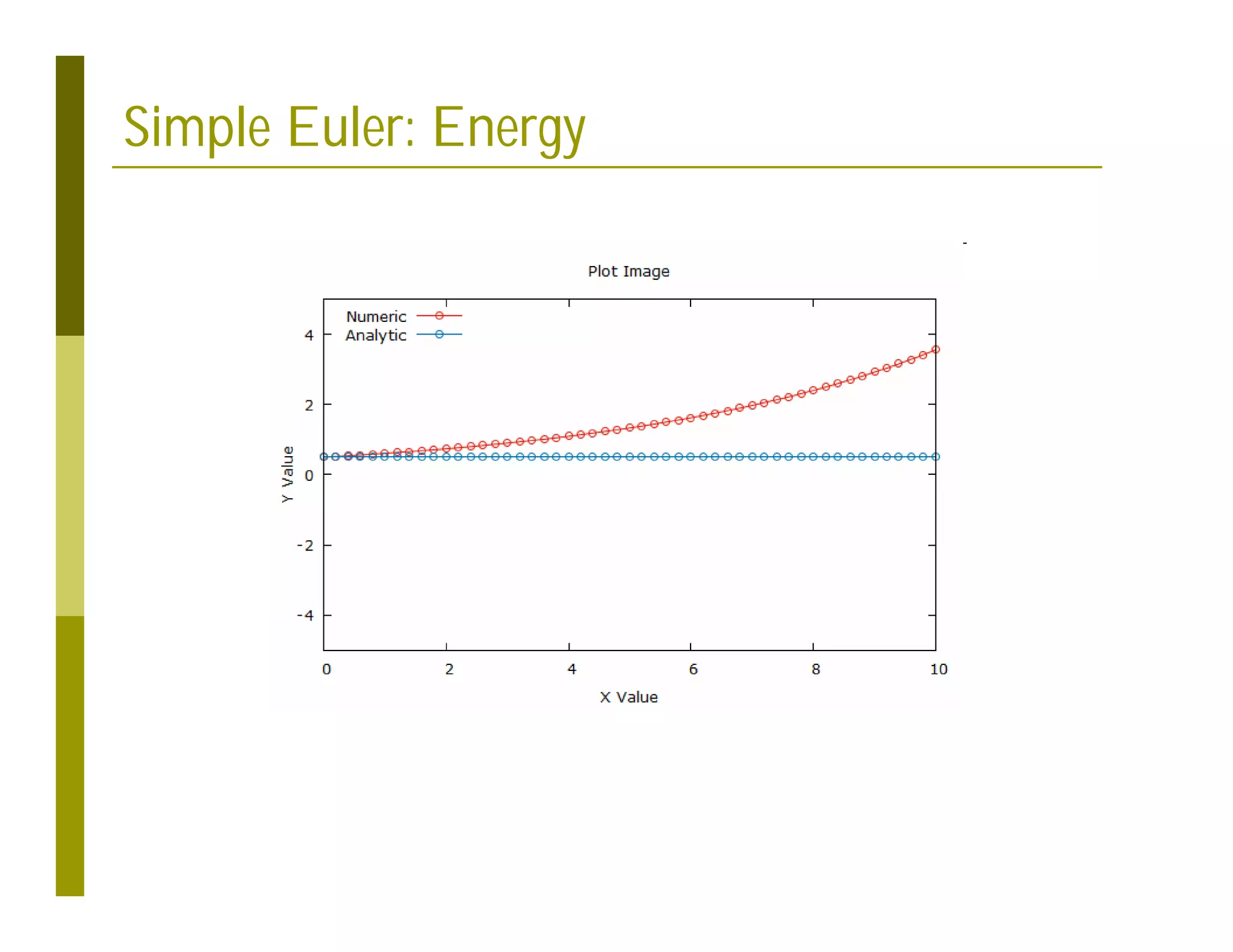
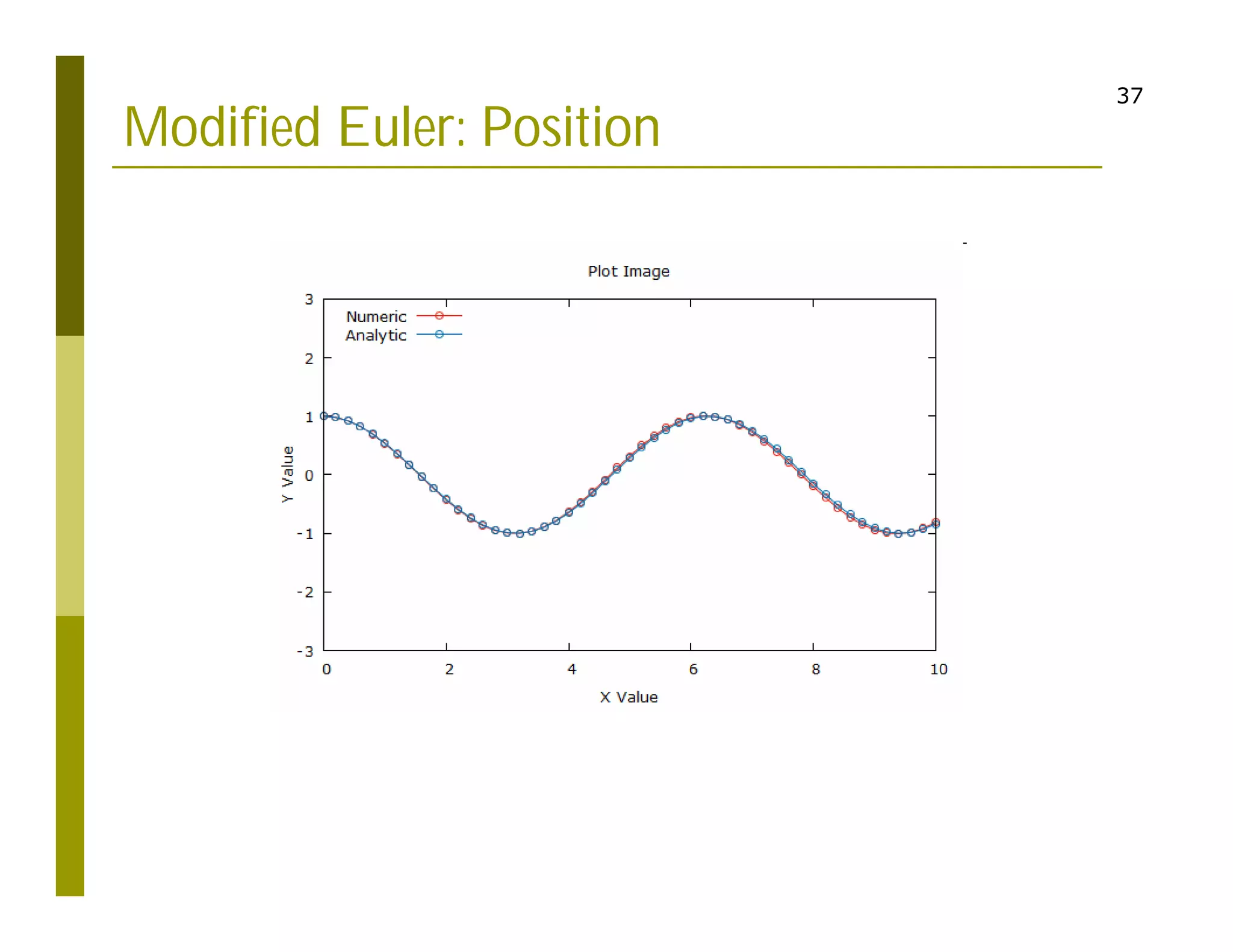
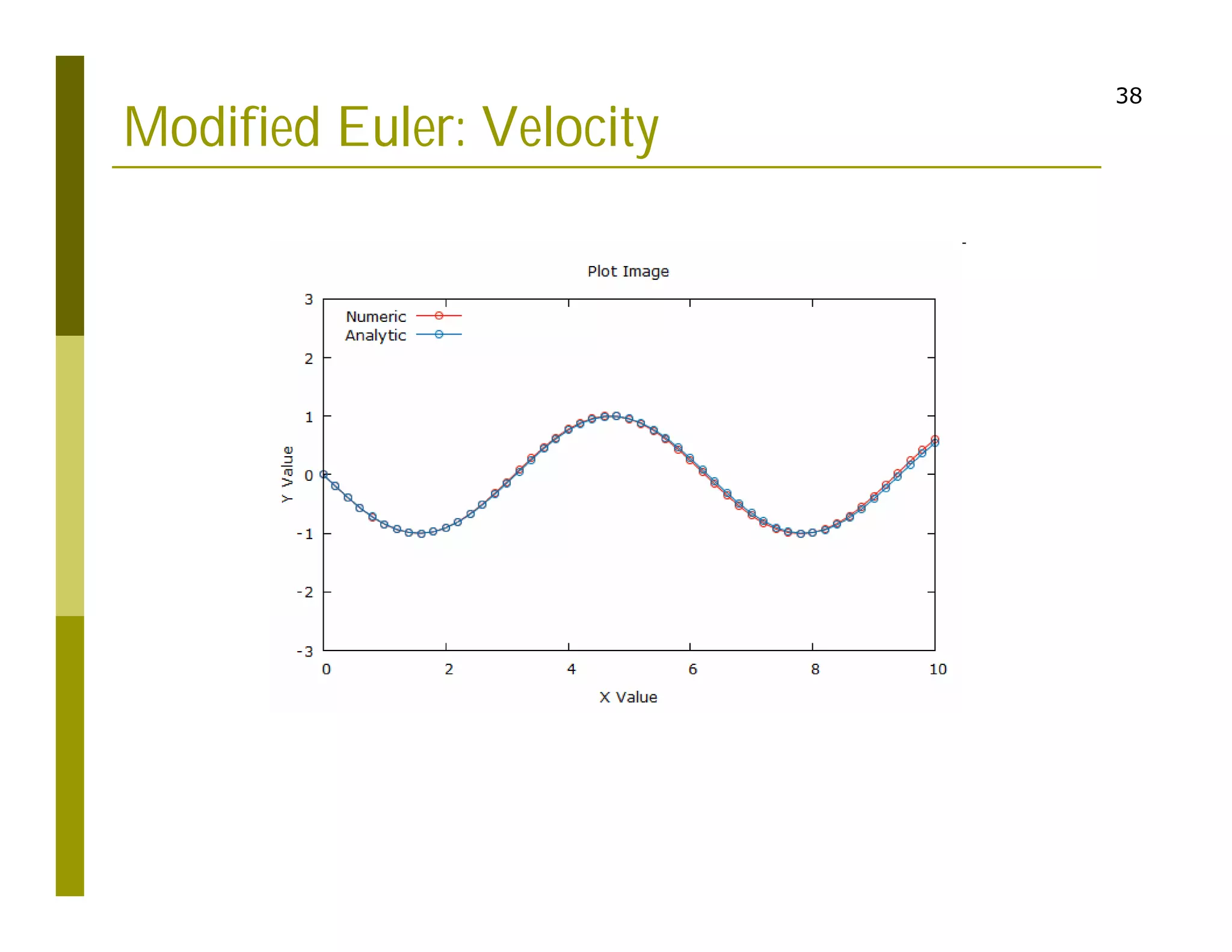
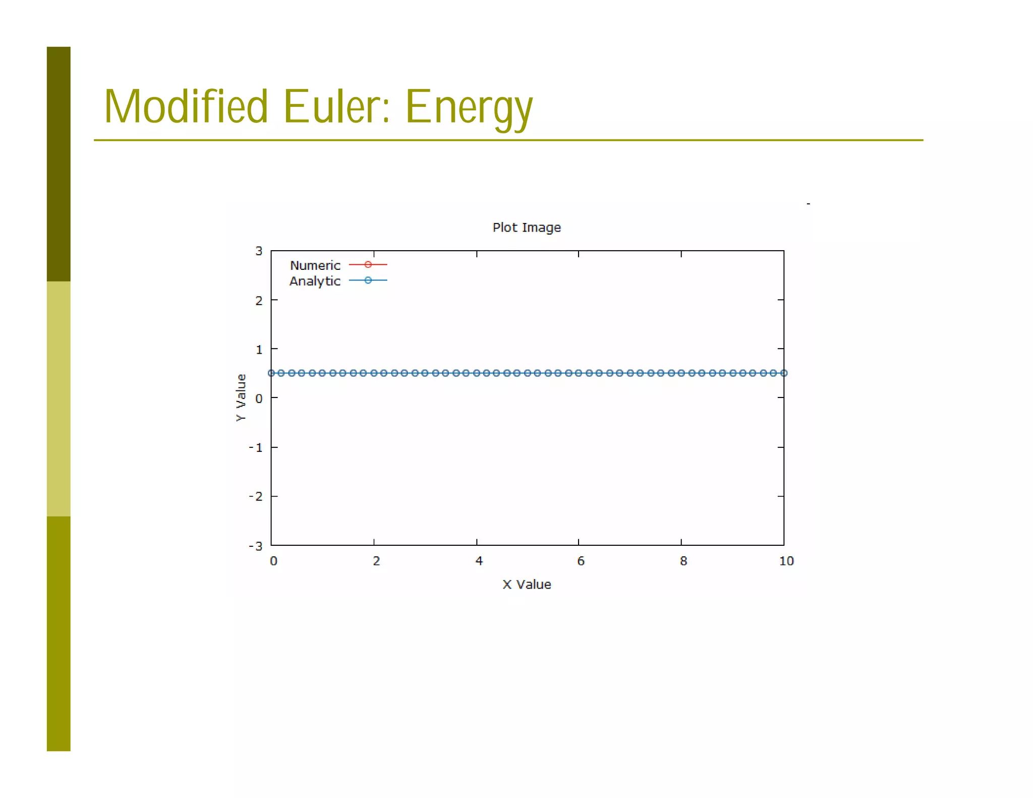
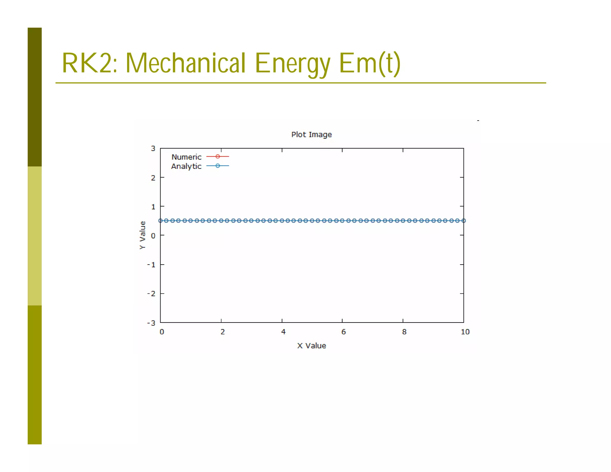
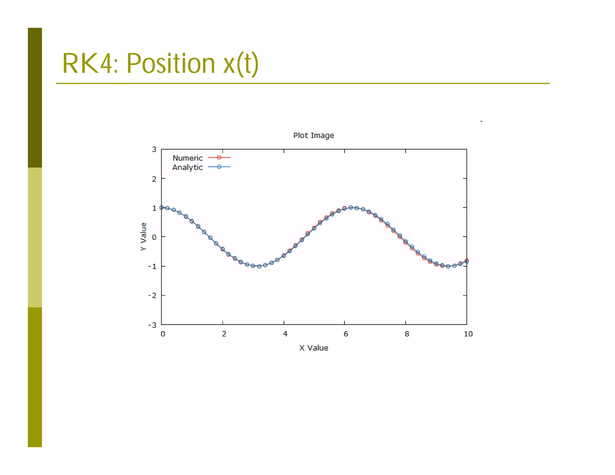
set title "Plot Image"
set xlabel "X Value"
set ylabel "Y Value"
set terminal wxt size 600,400 font "Verdana,10"
plot 'output.txt' using 2:3 title "Numeric" with linespoints pointtype 6 lw 1 lc 7,
'output.txt' using 2:4 title "Analytic" with linespoints pointtype 6 lw 1 lc 6](https://image.slidesharecdn.com/04eulerrk-211013005234/75/SPSF04-Euler-and-Runge-Kutta-Methods-32-2048.jpg)
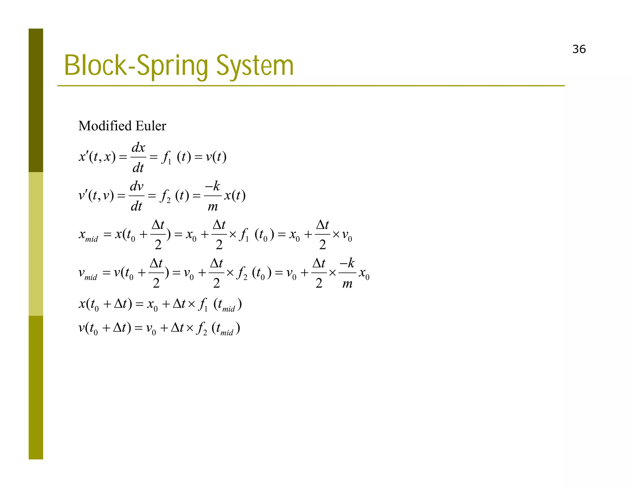
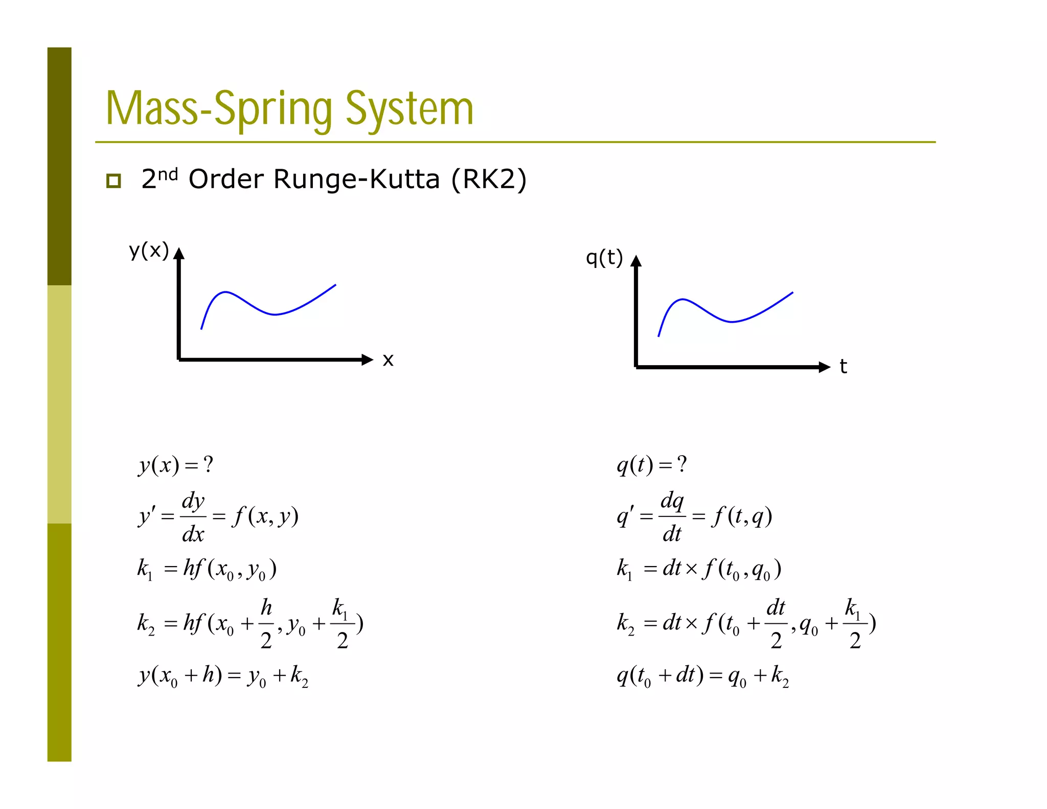

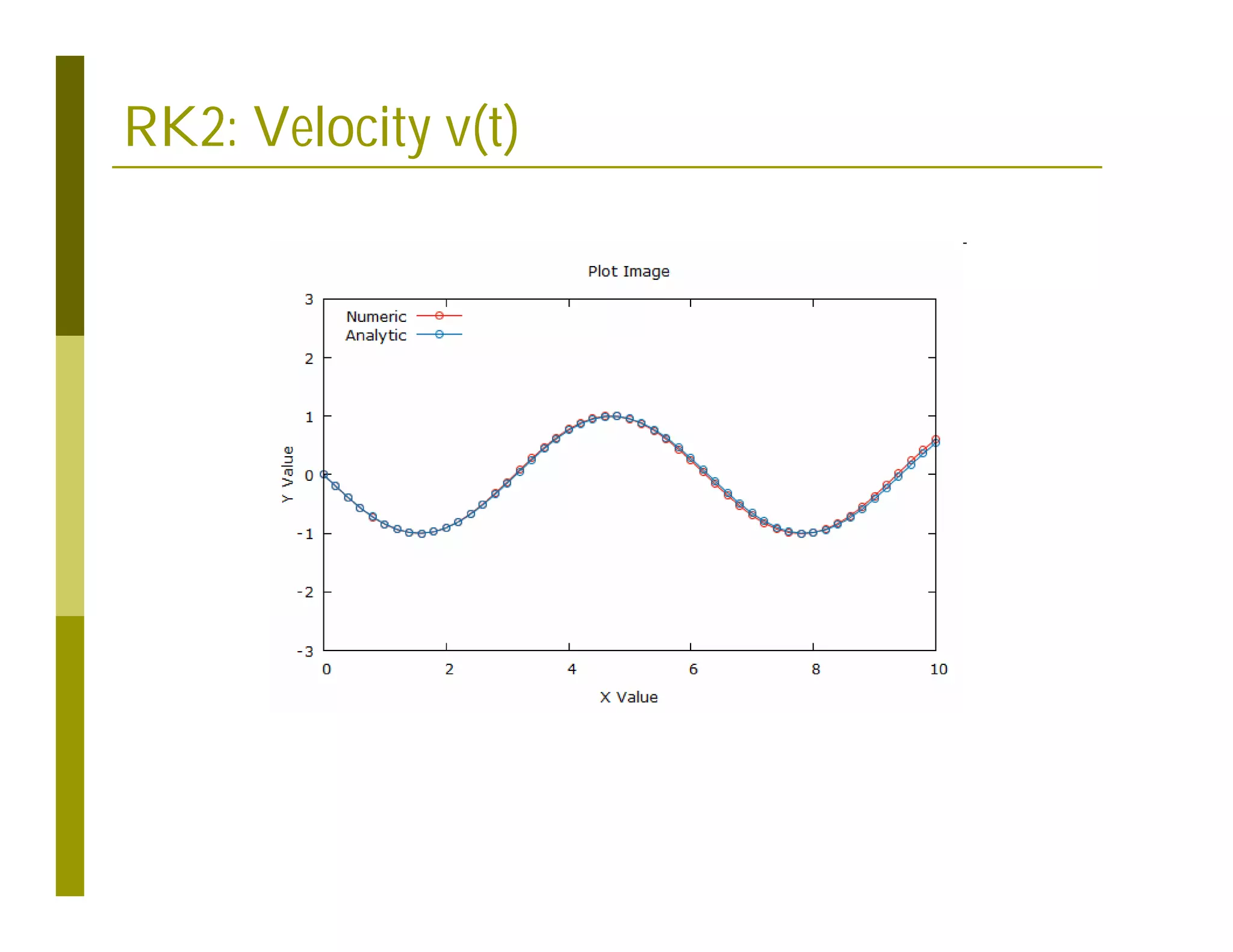
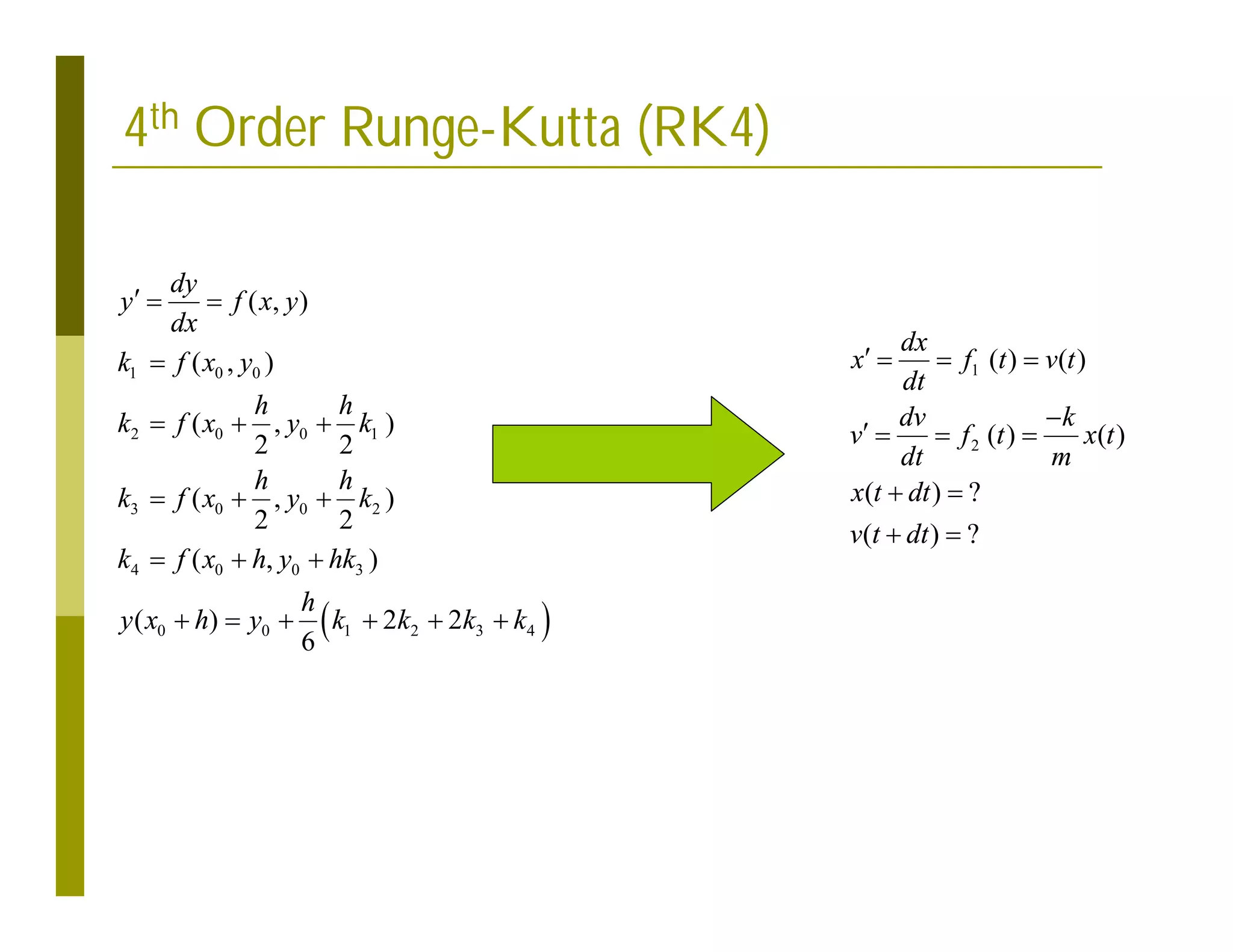
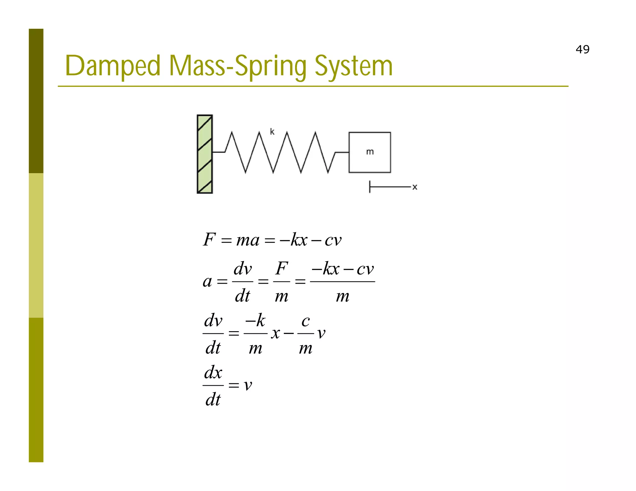
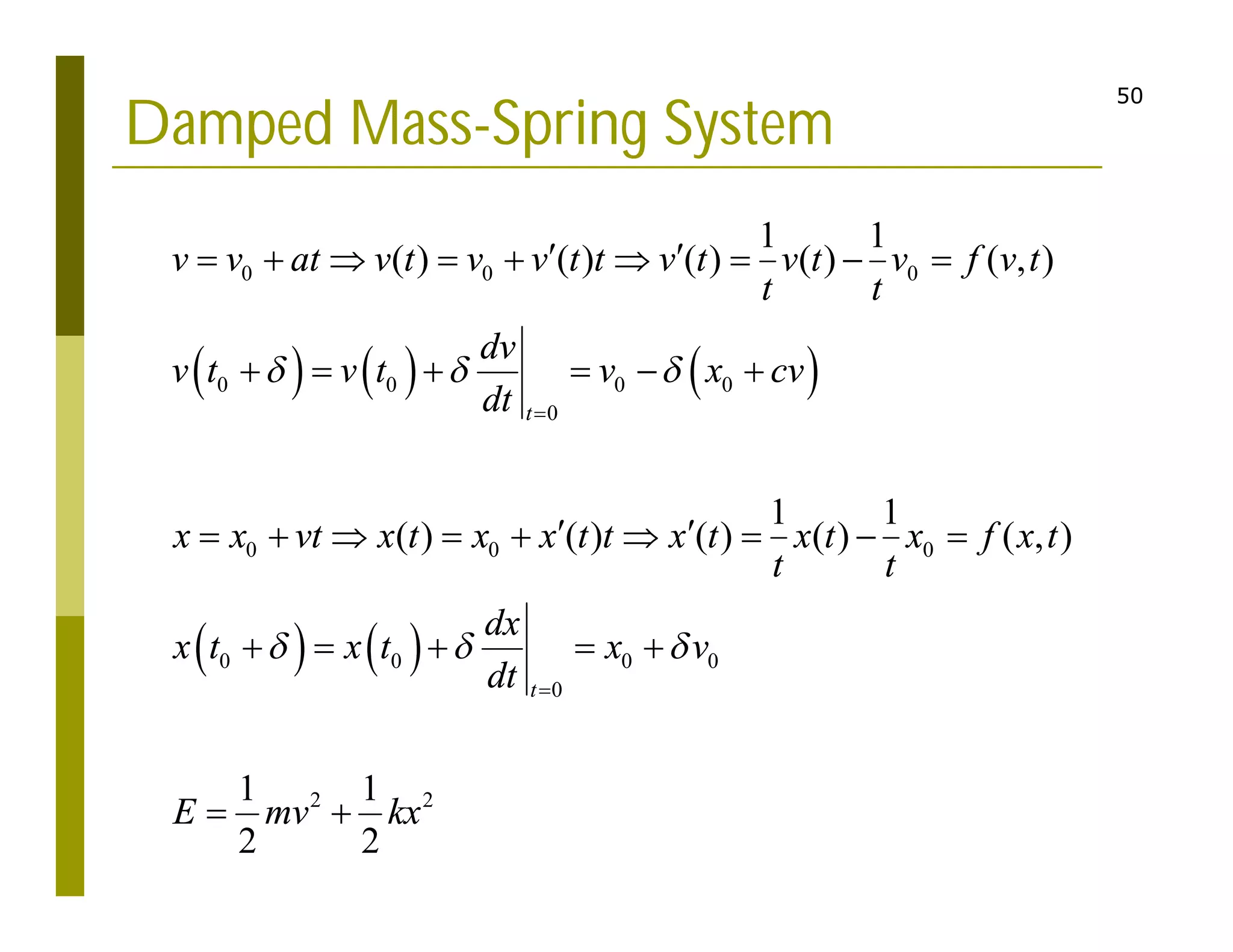
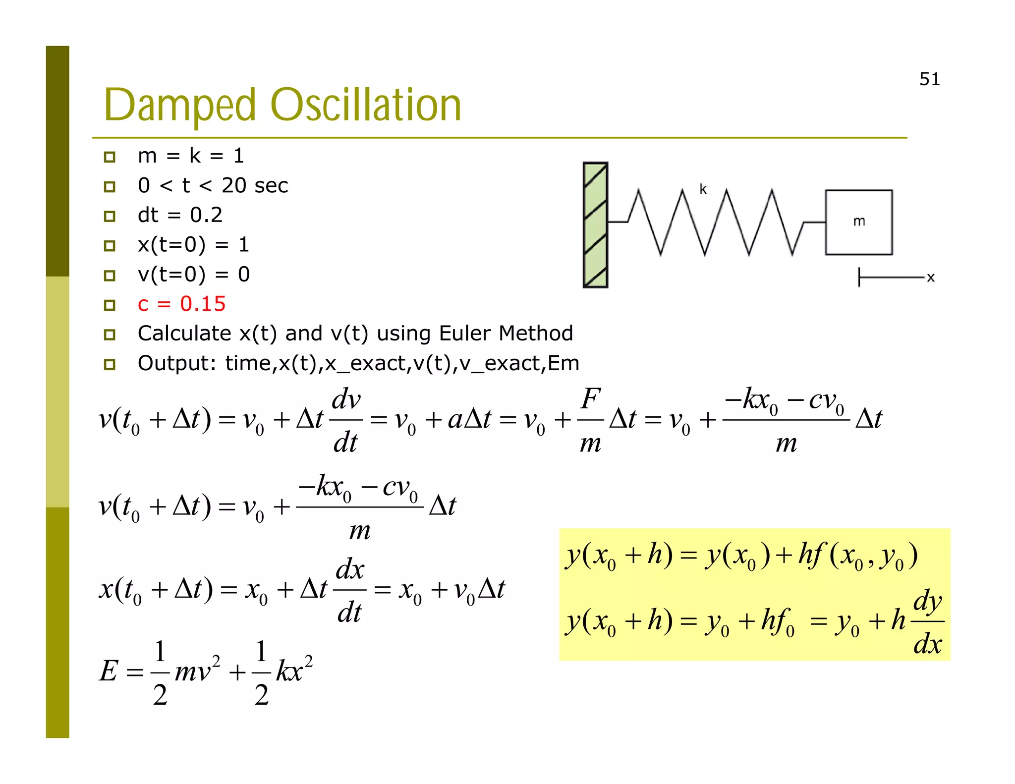
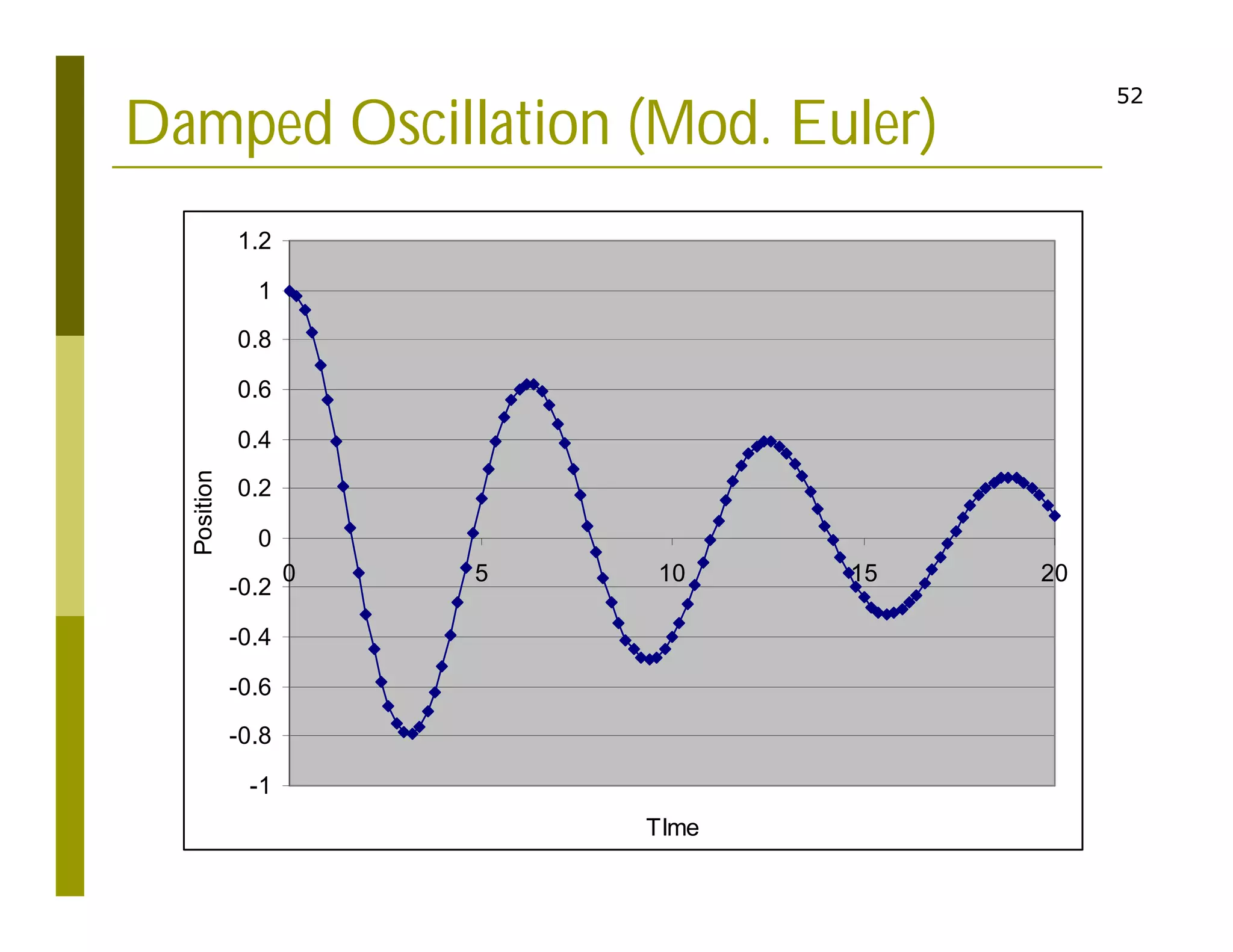
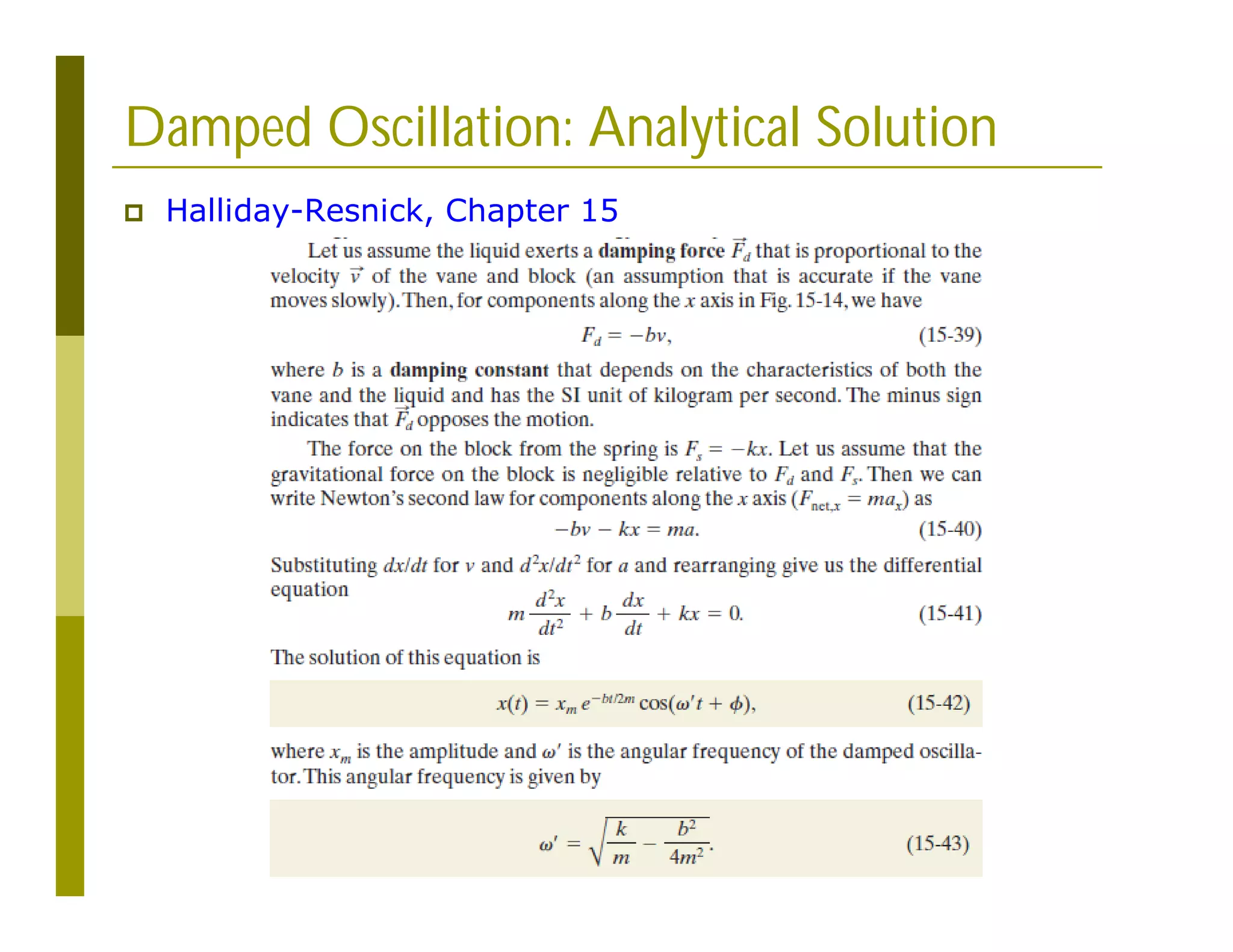

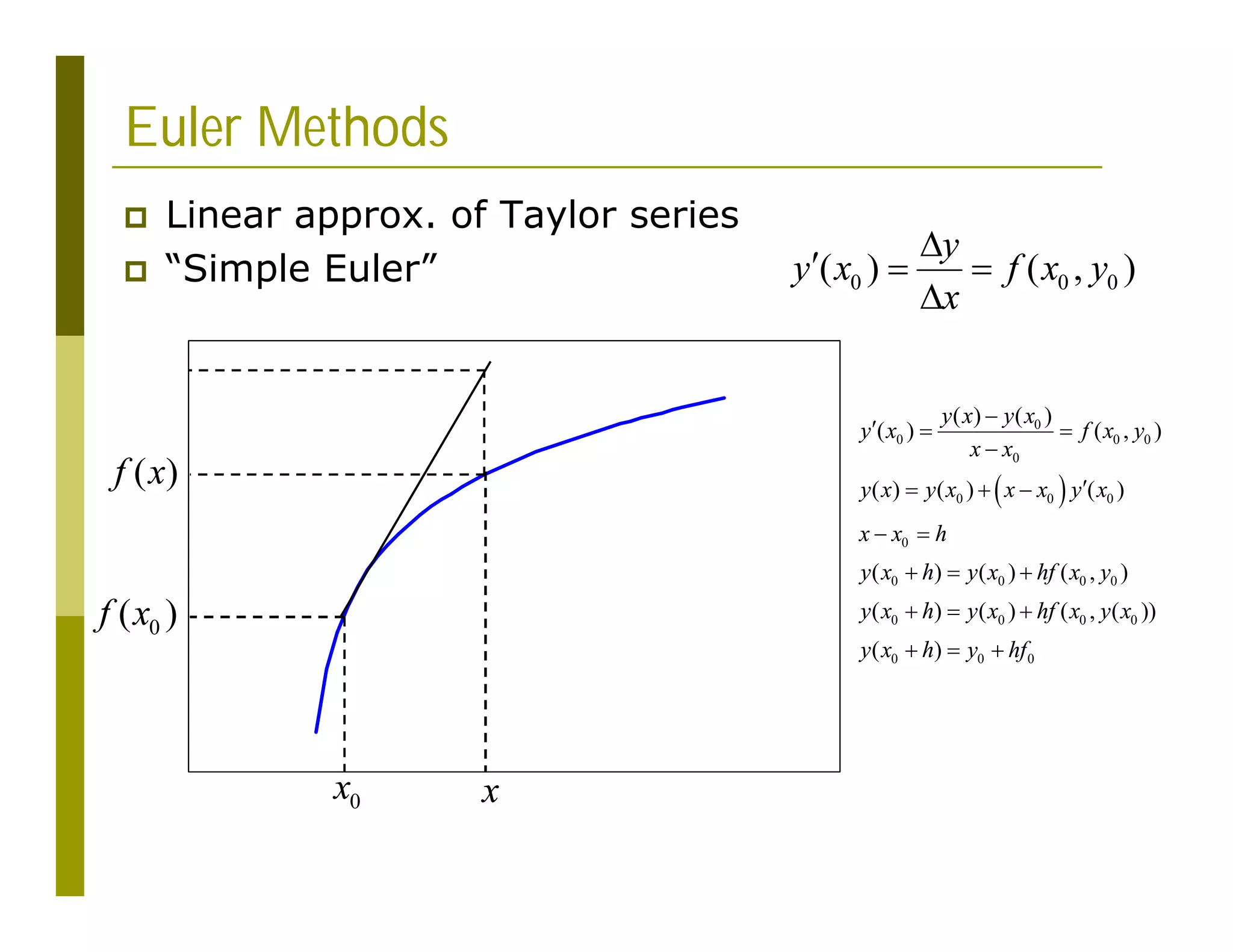
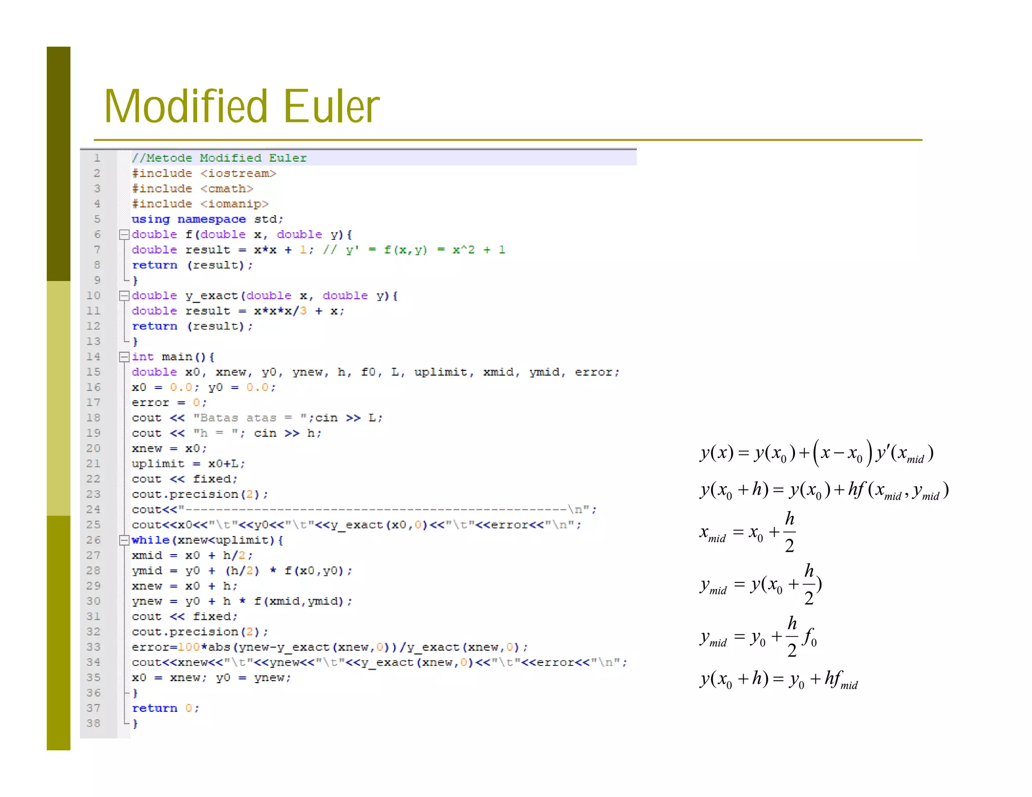
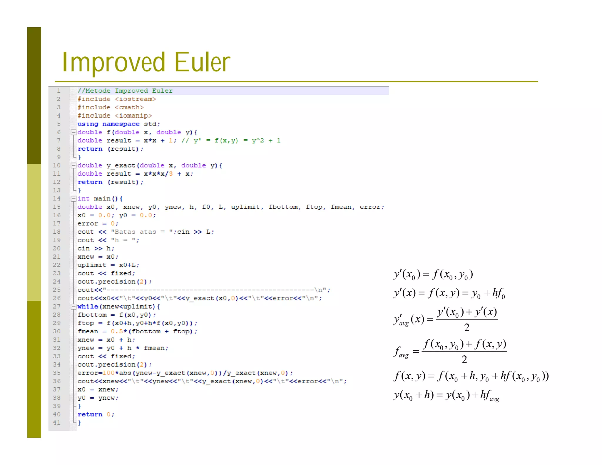
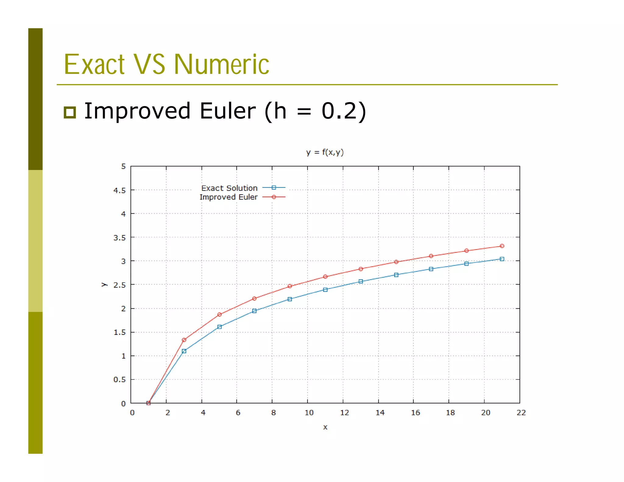
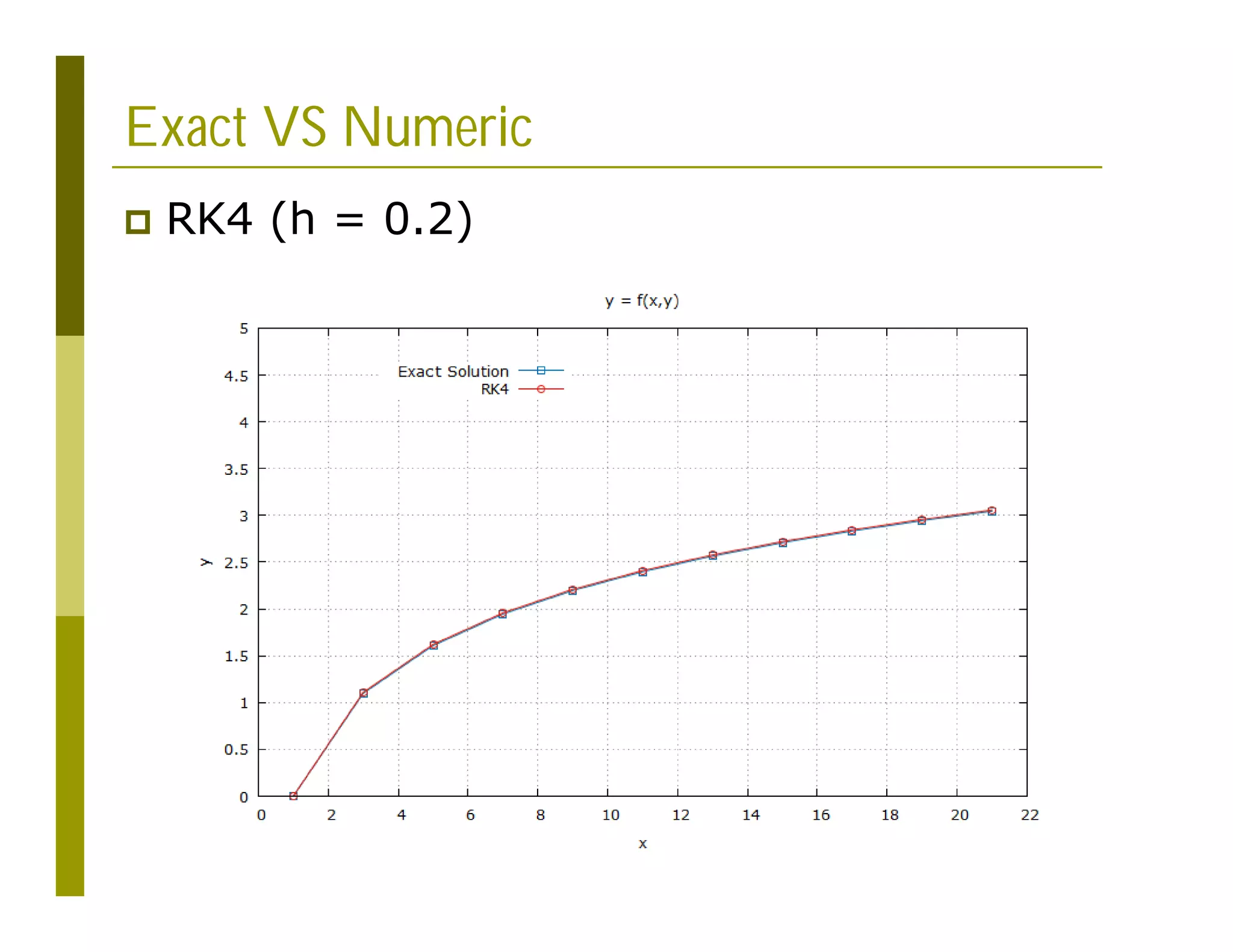
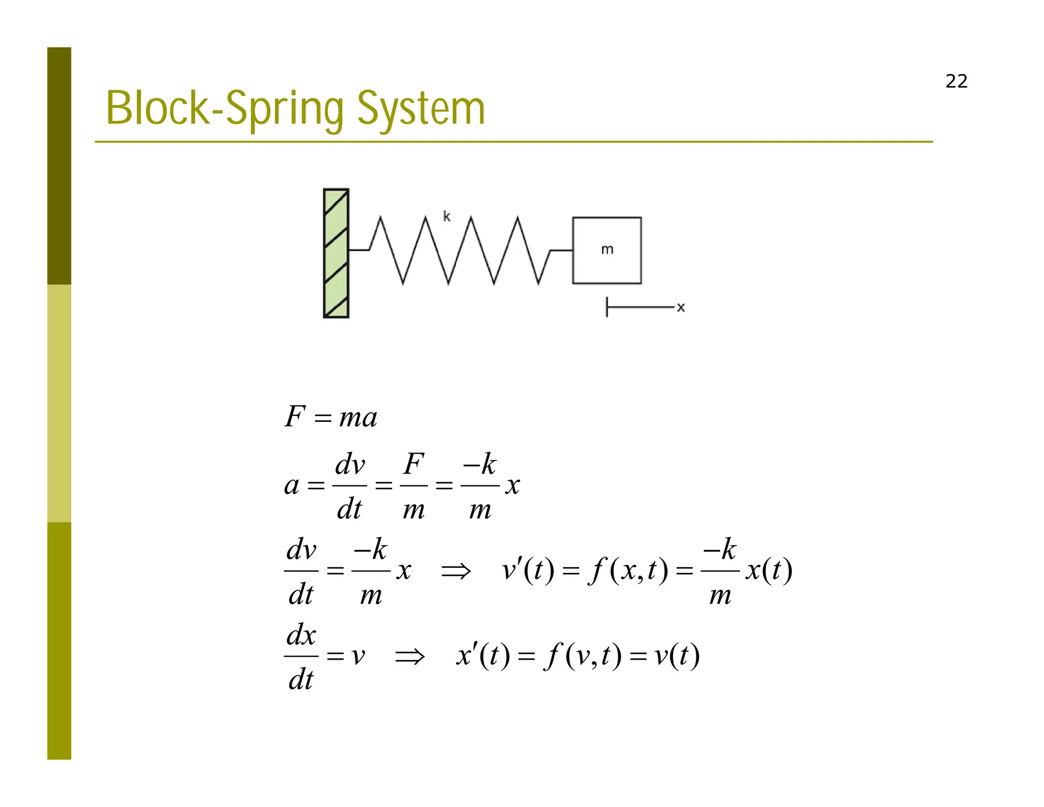
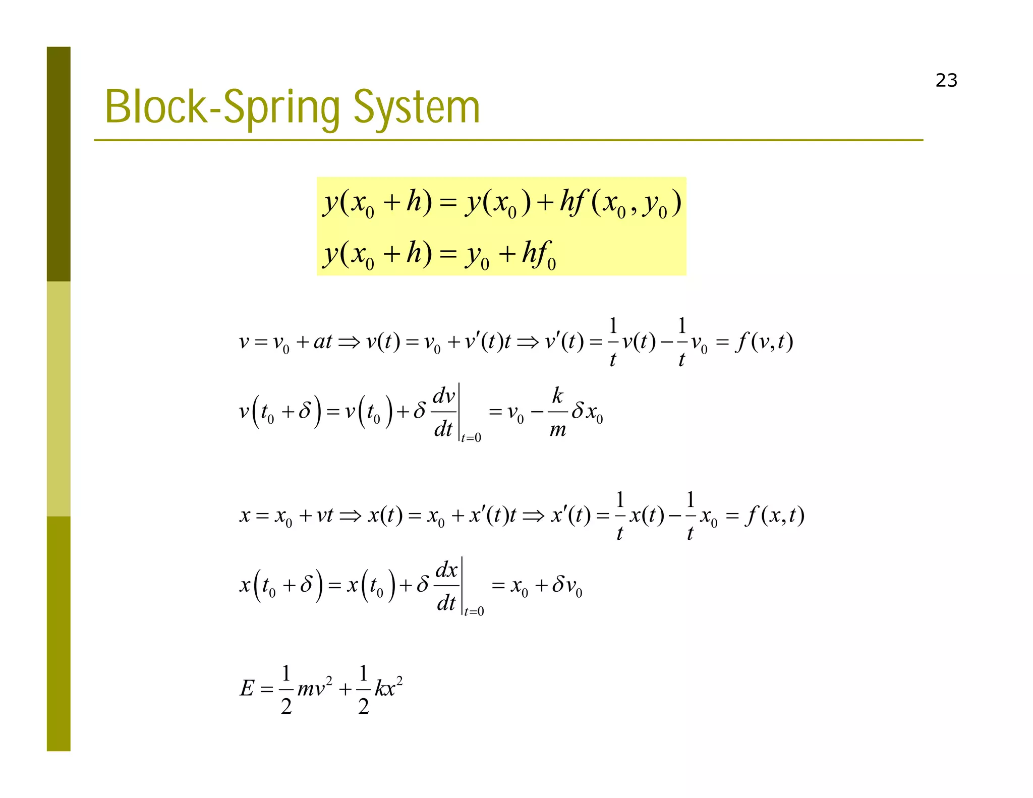
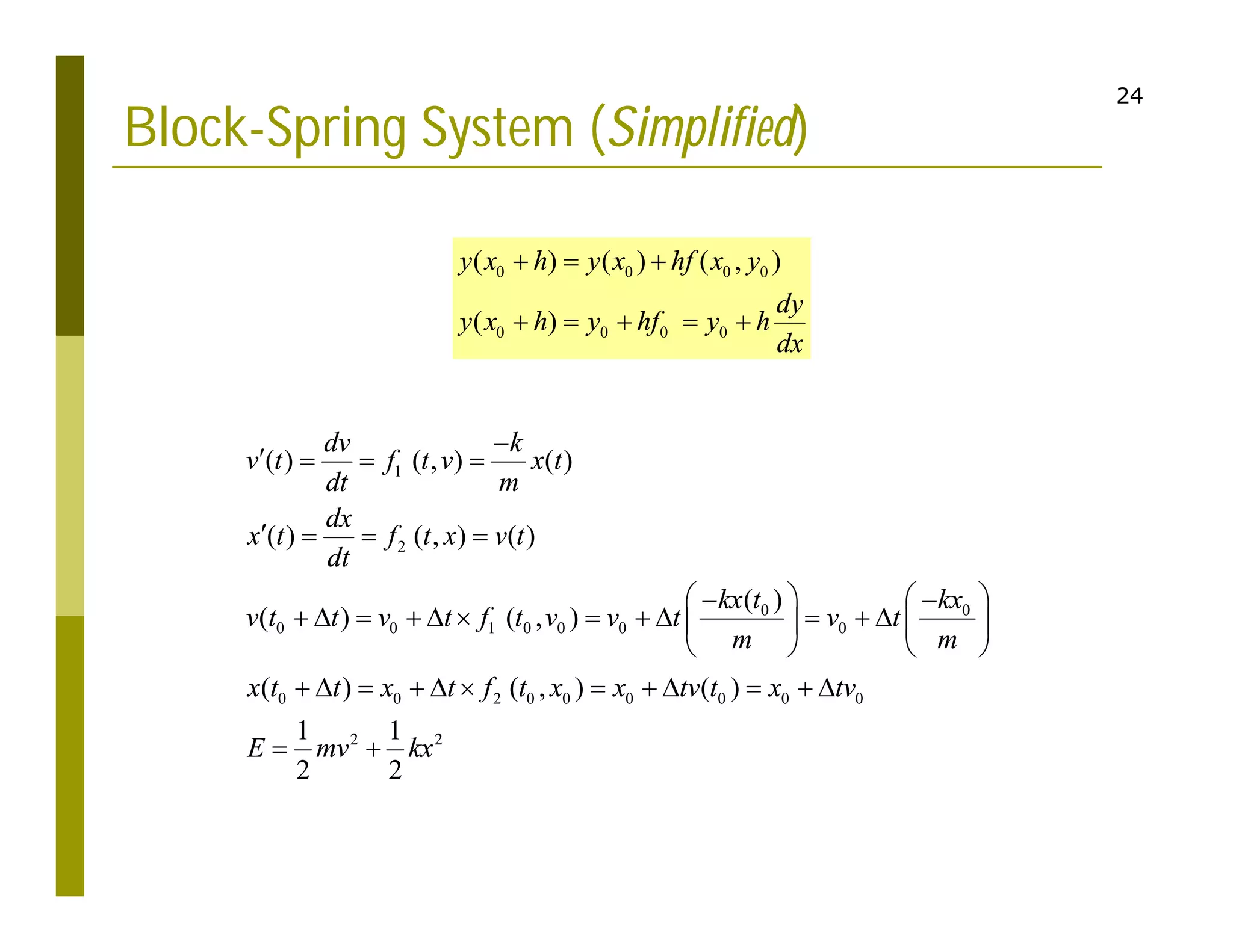
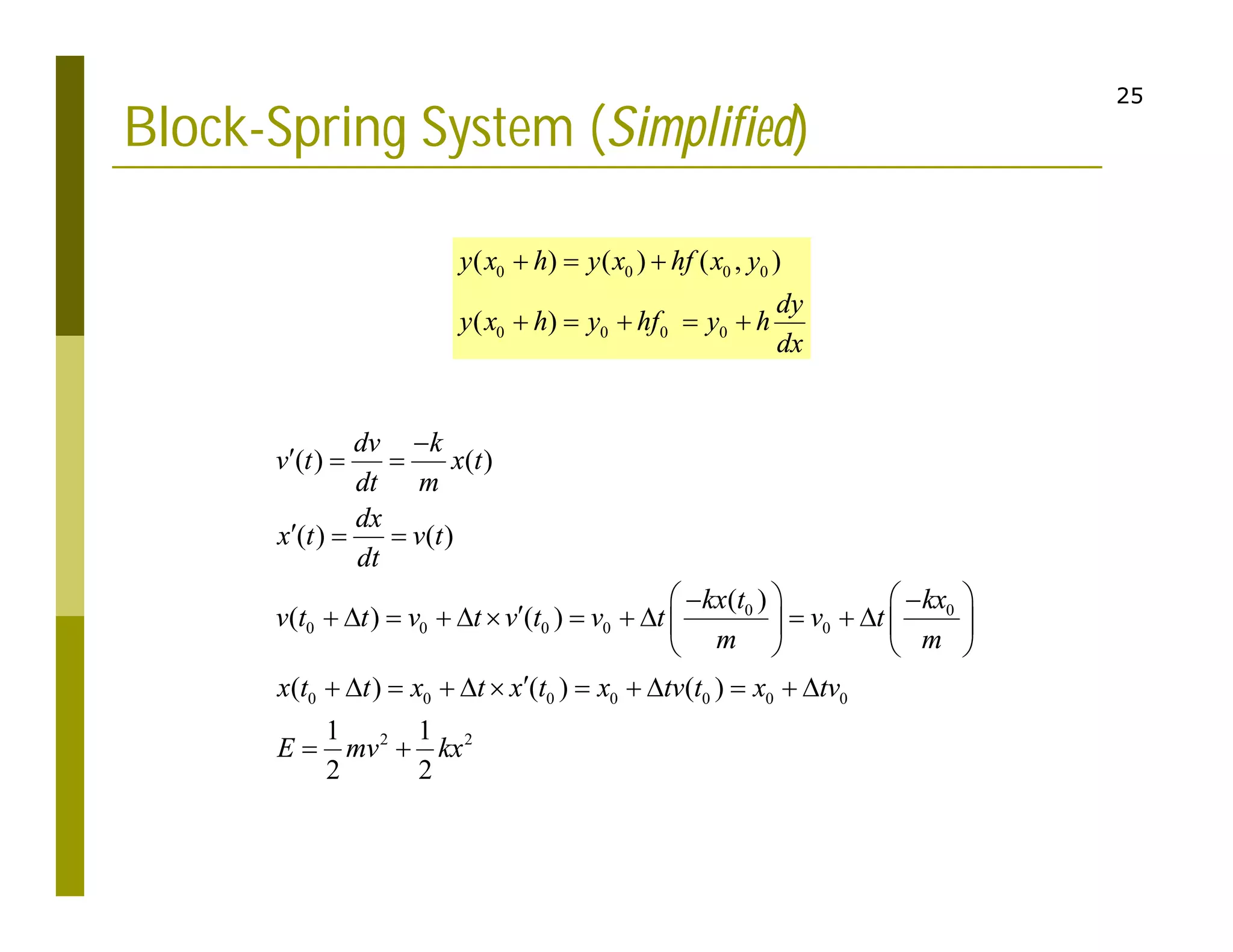
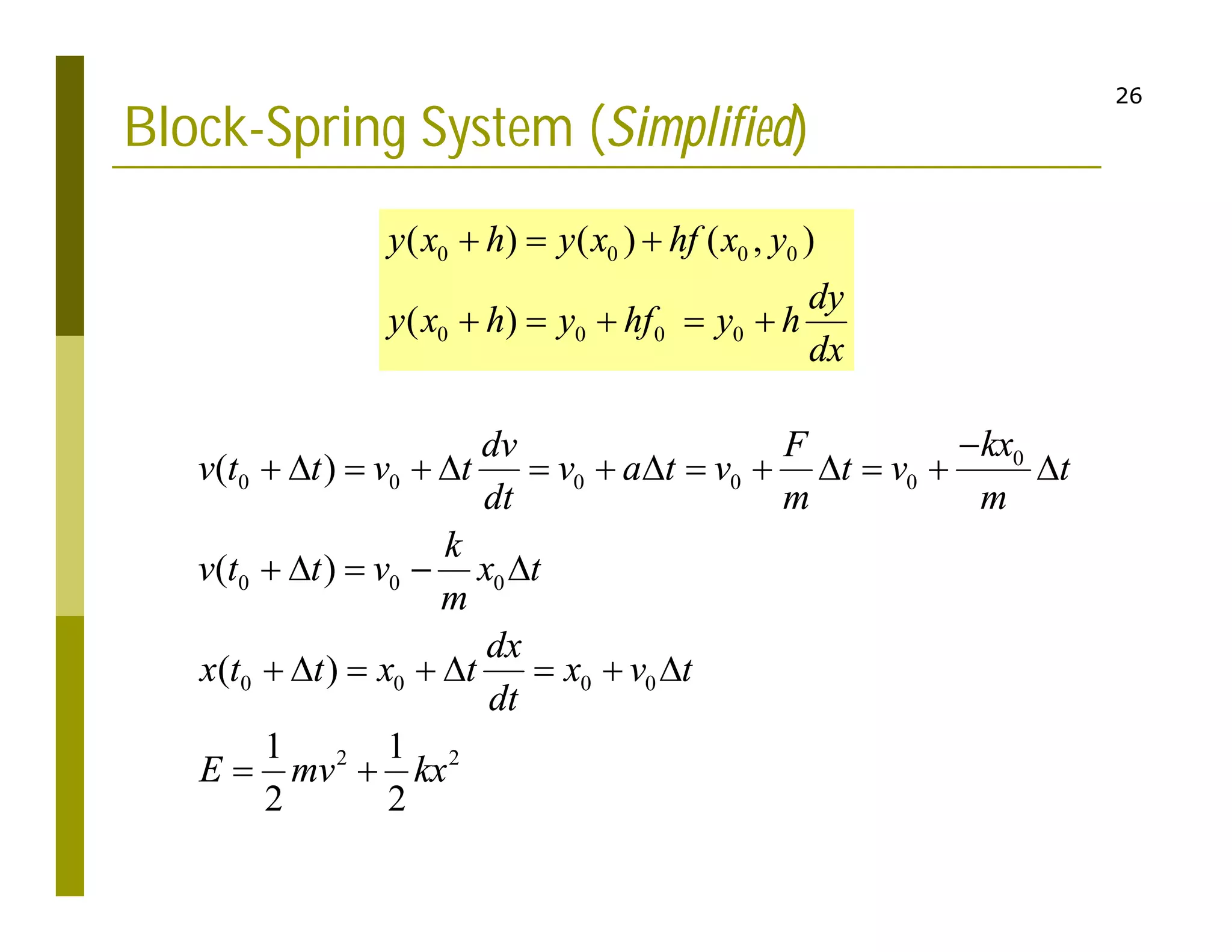
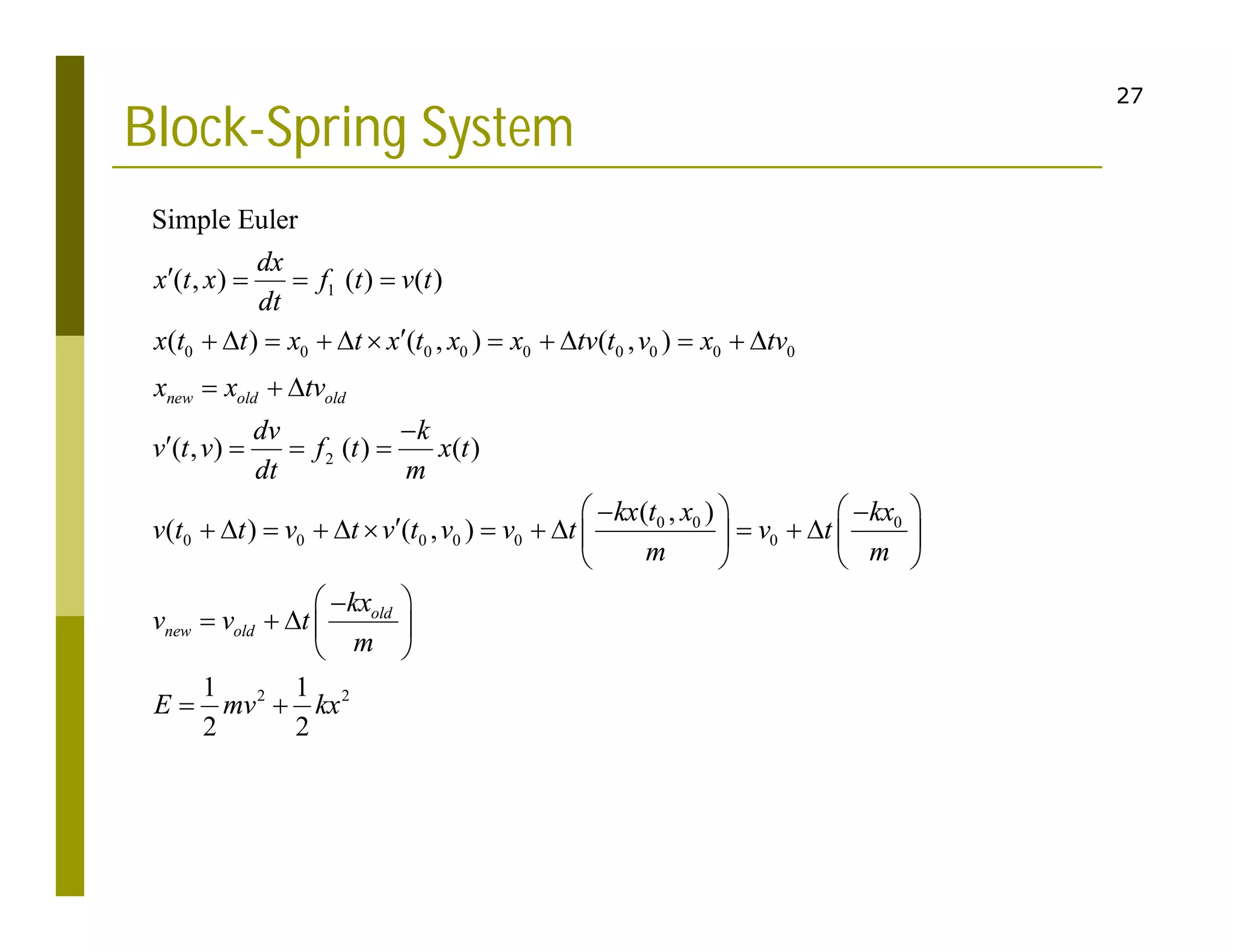
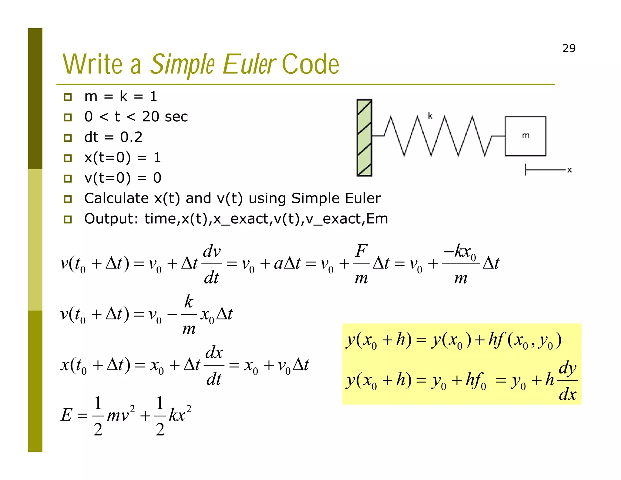
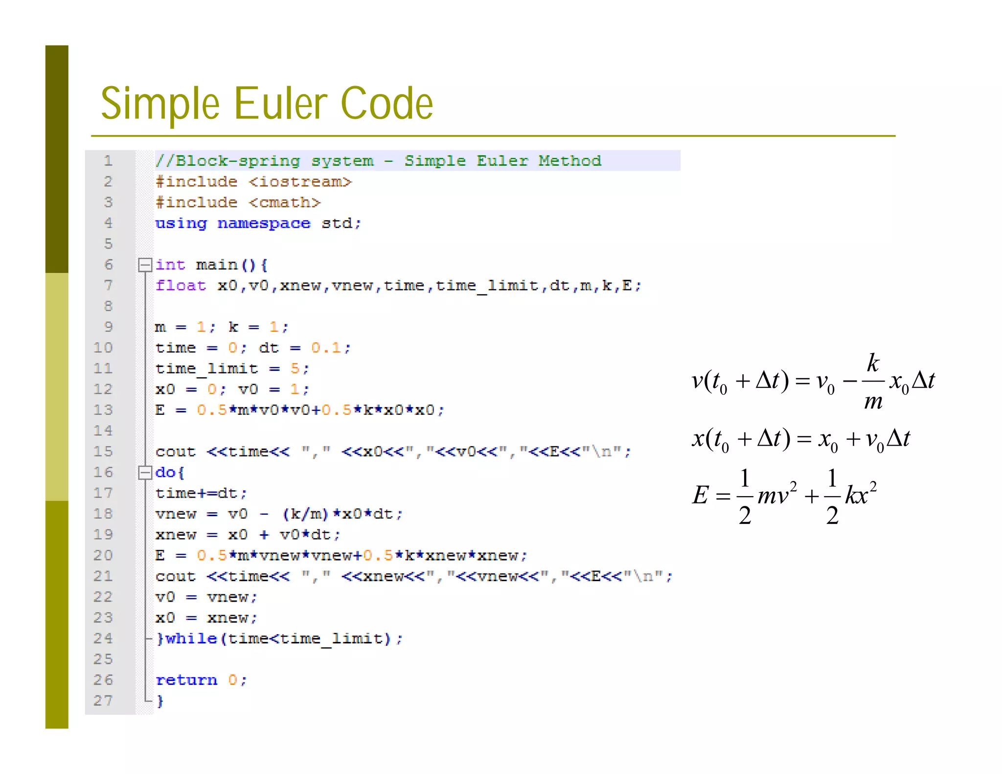
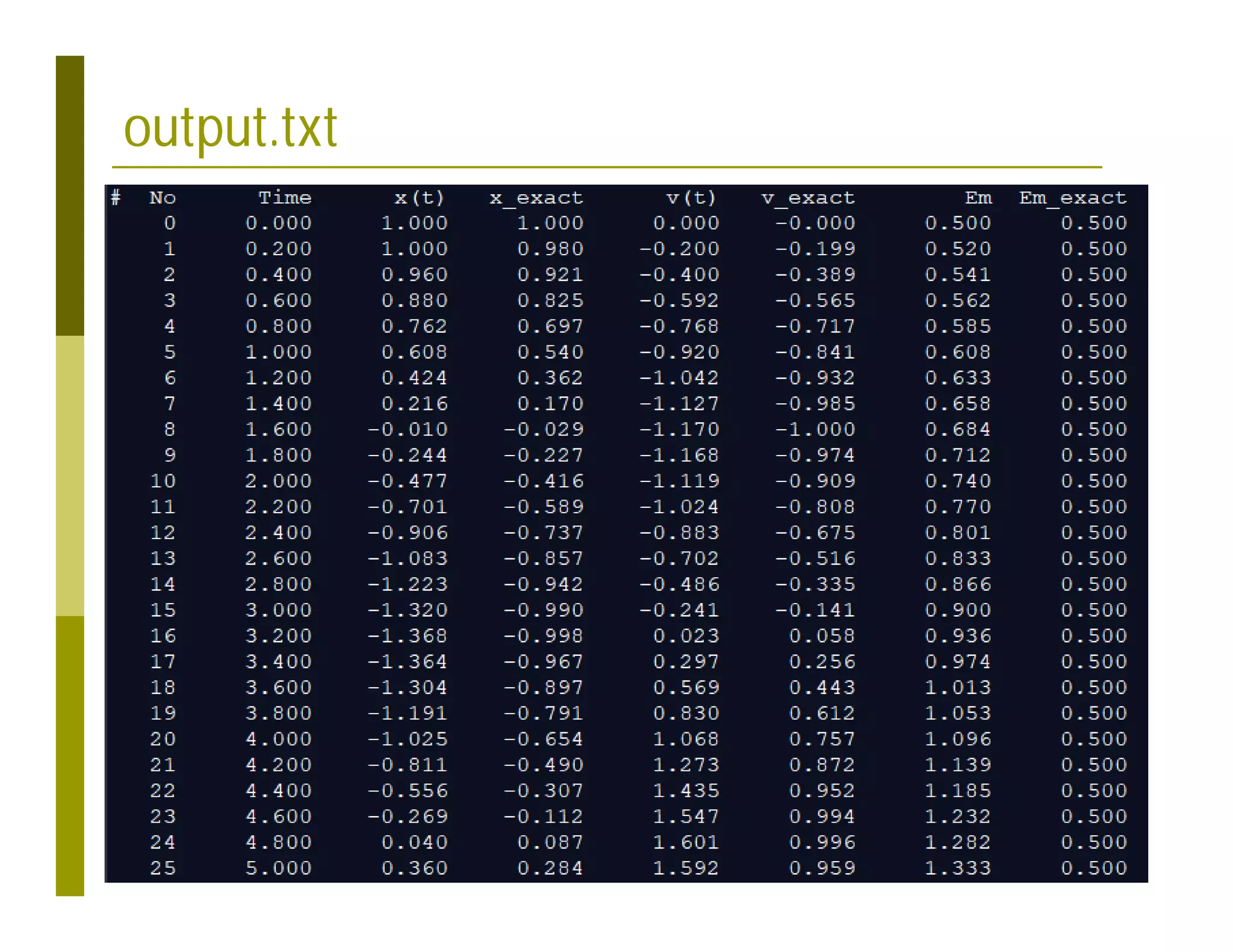
This document discusses numerical methods for solving ordinary differential equations (ODEs), including Euler methods, Runge-Kutta methods, and their application to problems in math and physics. It provides examples of using Euler's method and Runge-Kutta methods to solve ODEs describing a block-spring system. Code implementations of the Euler and Runge-Kutta methods are presented along with comparisons of numerical solutions to exact solutions.