![9
9
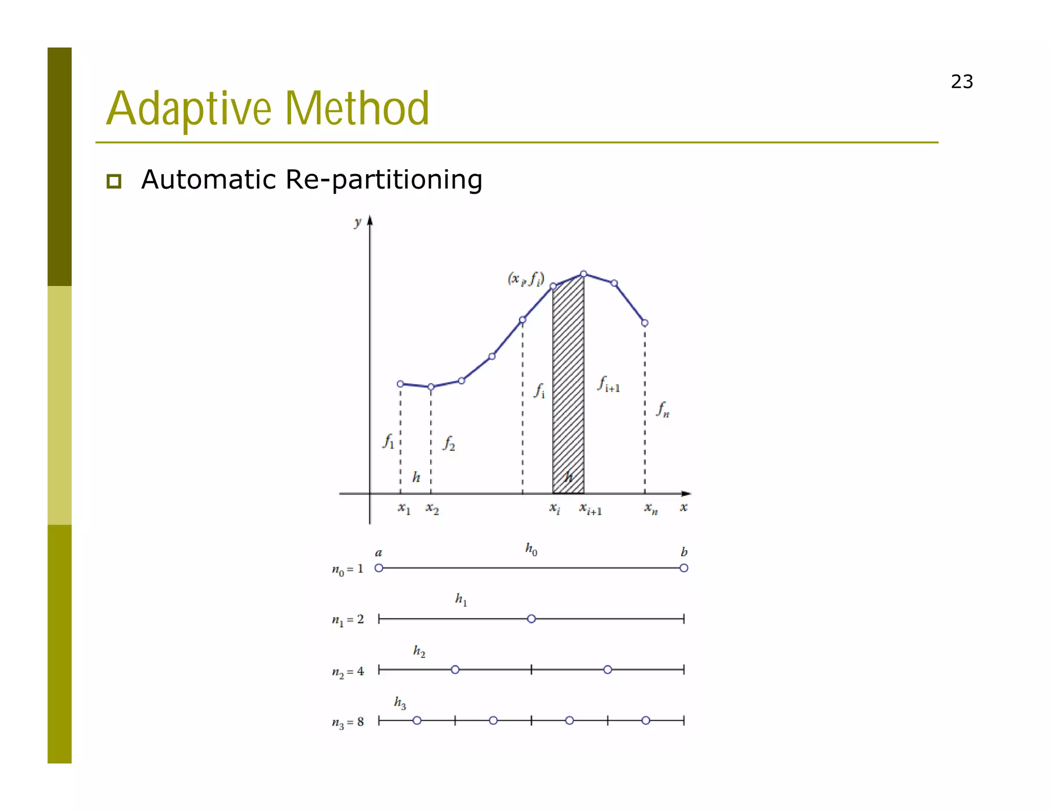
Numerical Integration
Definite integral of f(t) on
interval [a,b]
Analytic method: anti-
derivative
F where F’(t) = f(t)
Iab = F(b) – F(a)
( ) ( ) ( ) ( )
b
ab
a
F t I f t dt F b F a
](https://image.slidesharecdn.com/03integral-211013005136/75/SPSF03-Numerical-Integrations-9-2048.jpg)

![32
The Integral
2
2
1
5 sin ( )
x
x
I x x dx
Gnuplot
set xrange [0:10]
set xrange [0:20]
plot x*(sin(x))**2](https://image.slidesharecdn.com/03integral-211013005136/75/SPSF03-Numerical-Integrations-32-2048.jpg)
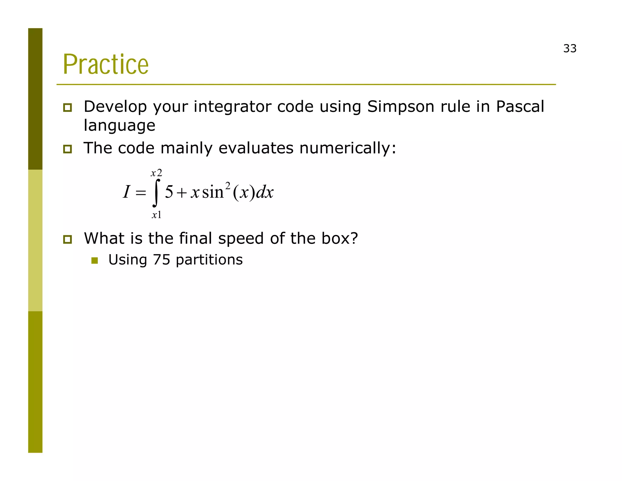

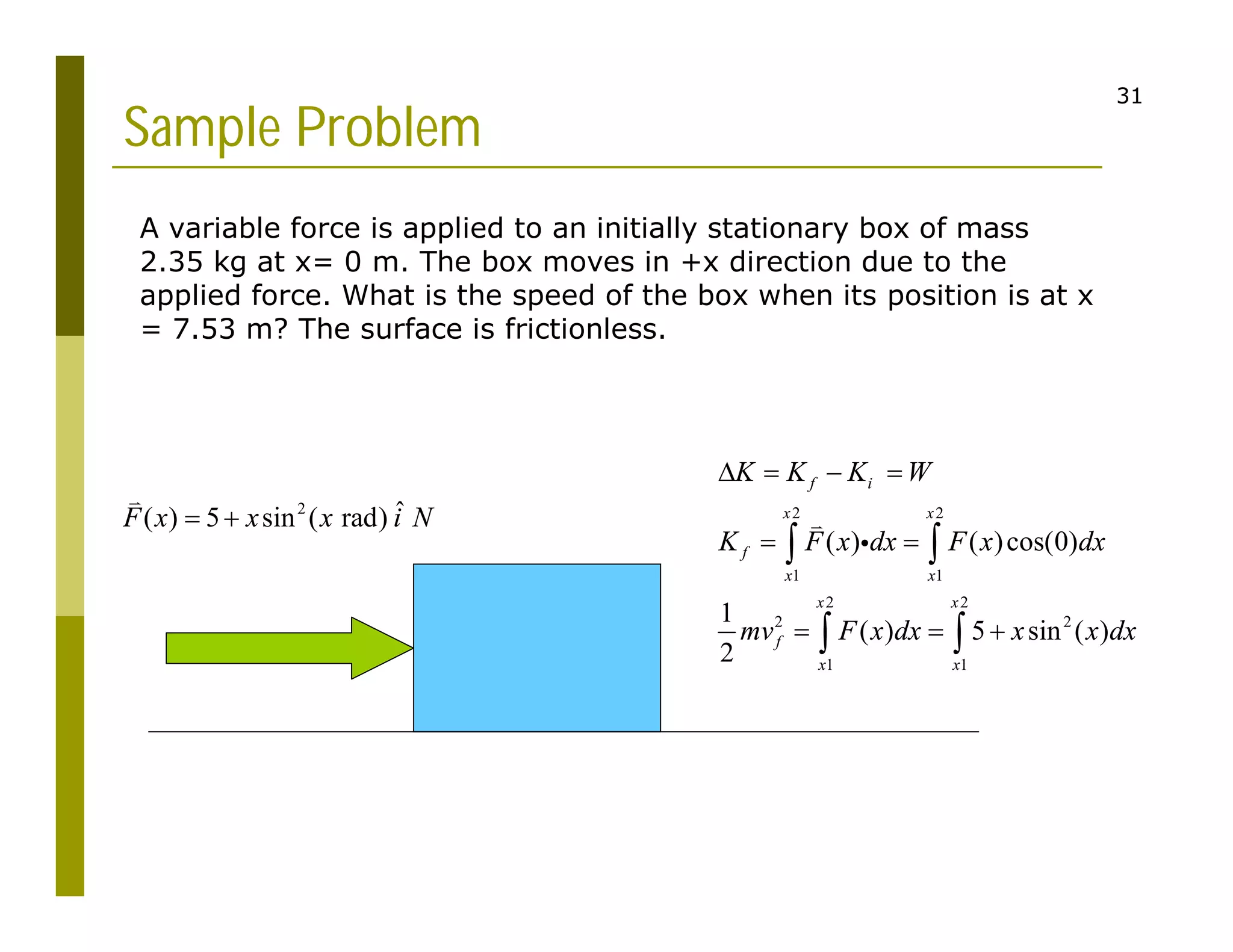
1. The document discusses numerical integration techniques for approximating definite integrals that cannot be solved analytically. It covers basic techniques like the rectangle, midpoint, and trapezoid rules as well as more accurate techniques like Simpson's rule. 2. Examples are provided to demonstrate calculating definite integrals numerically to approximate values like the natural logarithm of numbers. The document also introduces Monte Carlo integration techniques using random sampling. 3. As an example problem, the document calculates the final speed of a box moving under a time-varying force using numerical integration over the integral expression for work. The Simpson's rule is identified as an approach to implement in a programming code to solve this example.