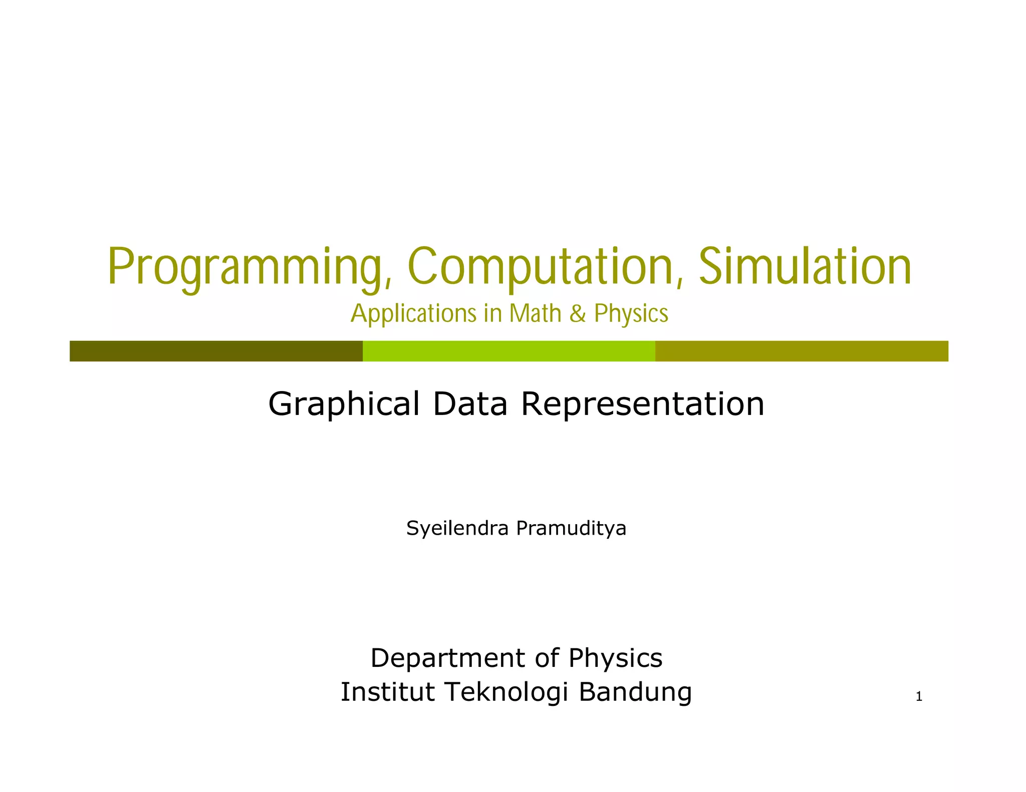
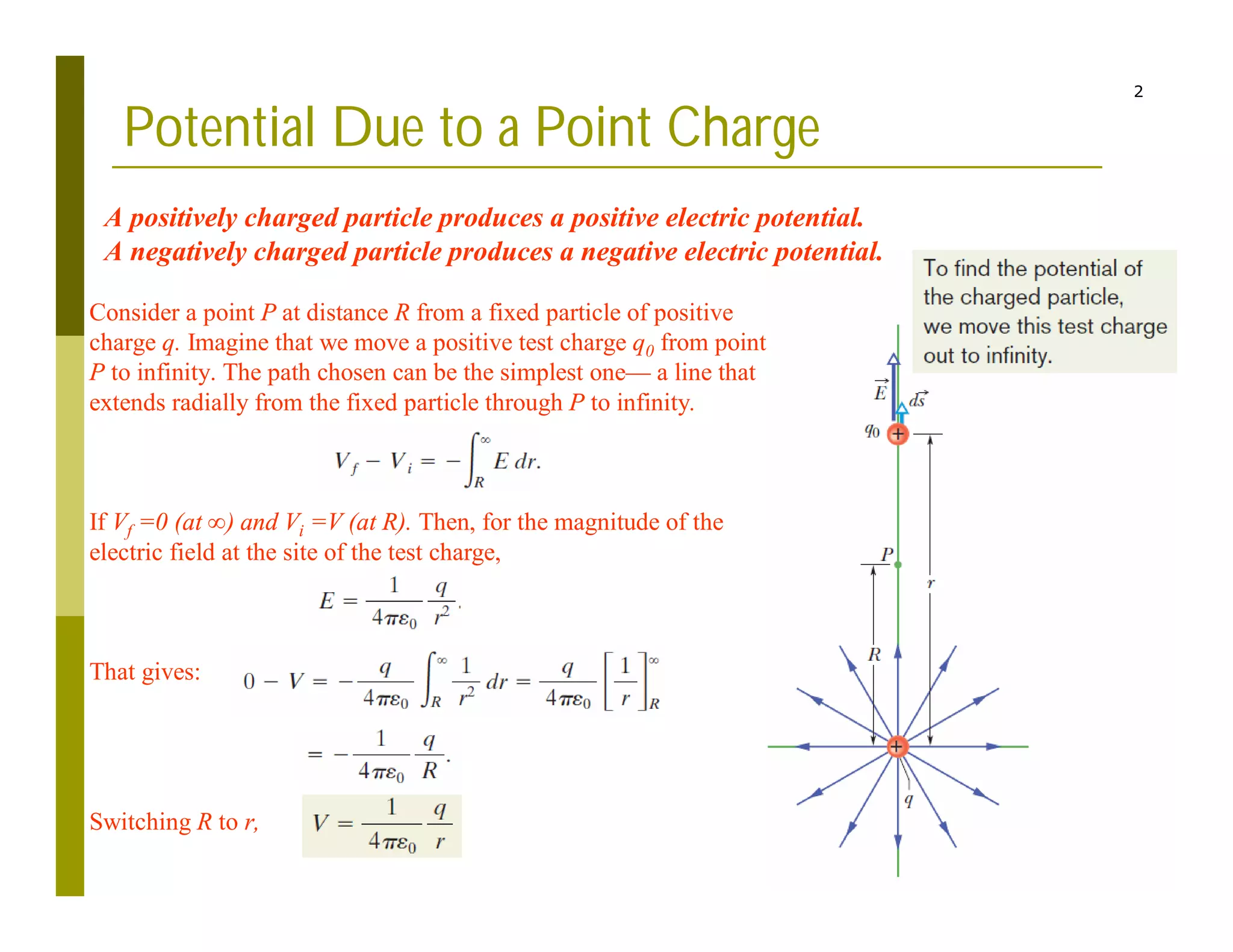
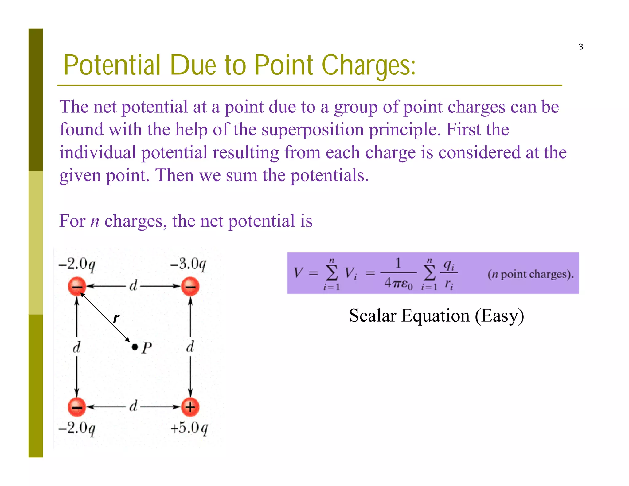
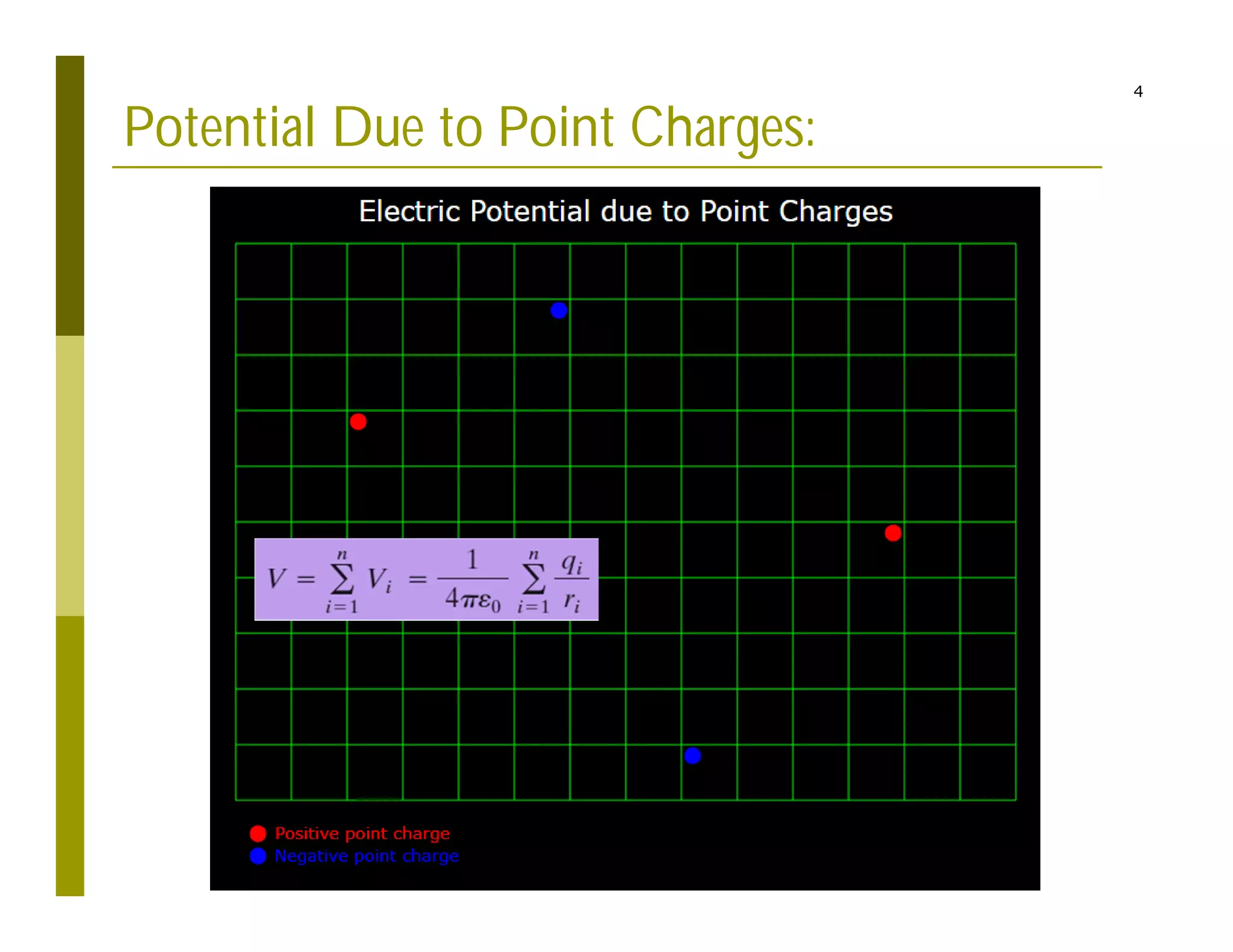
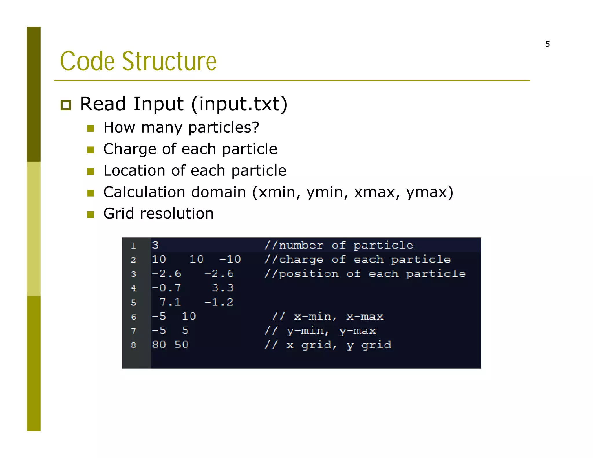
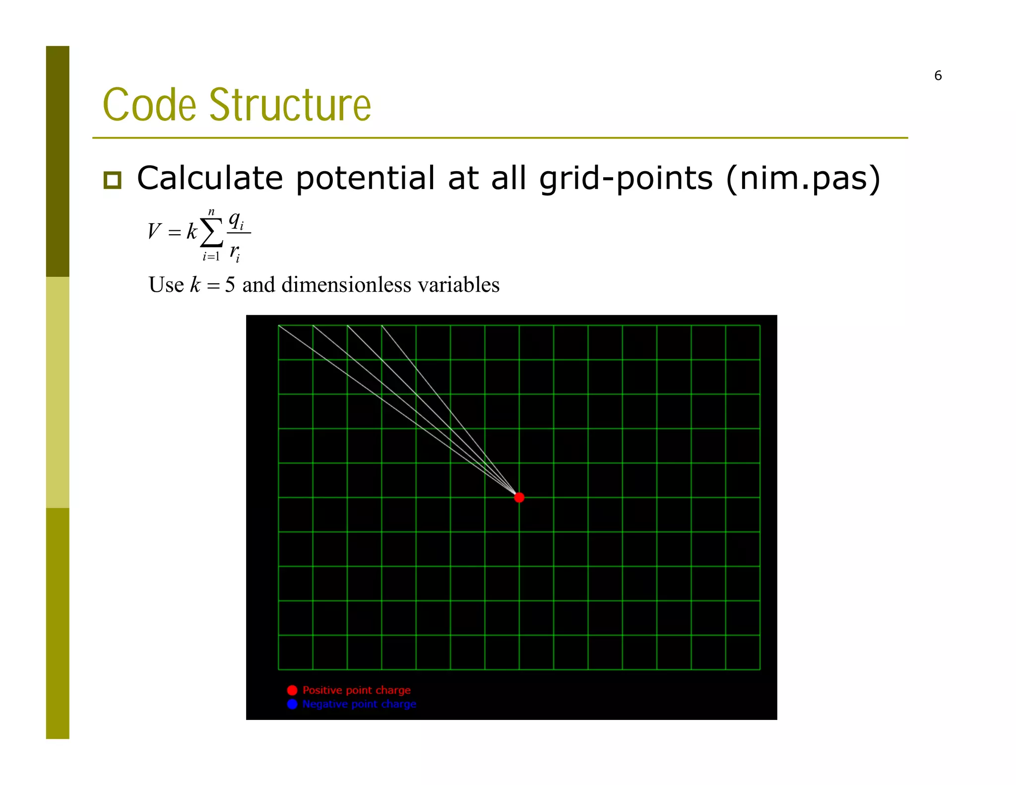
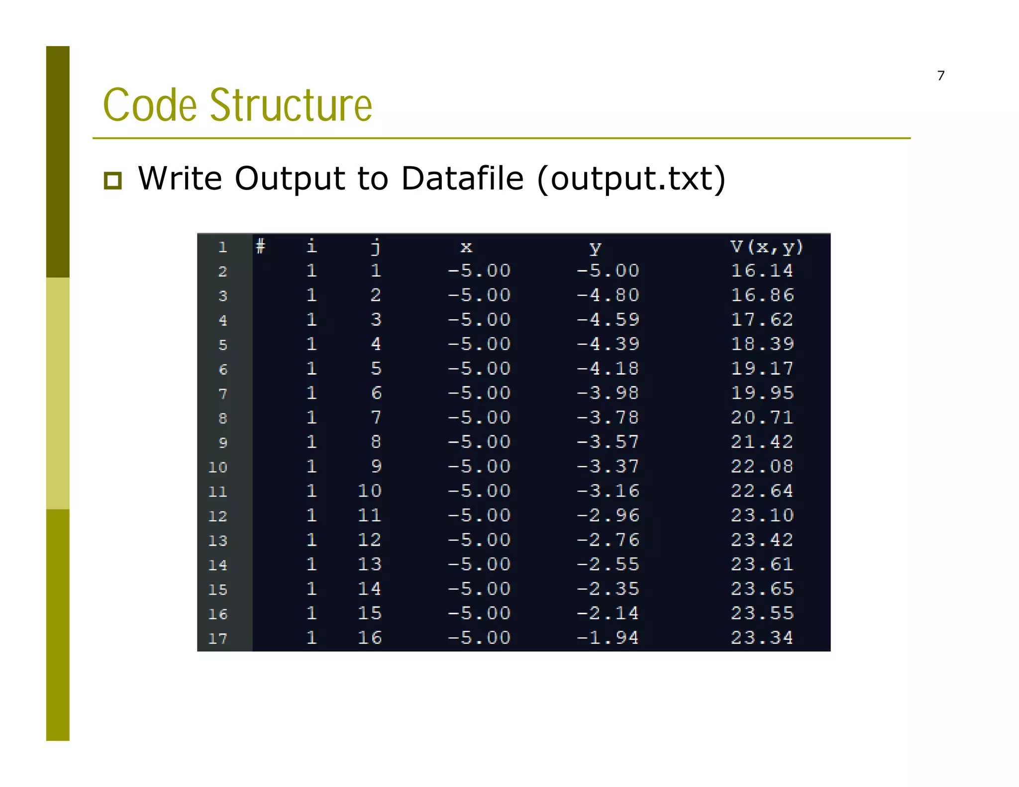
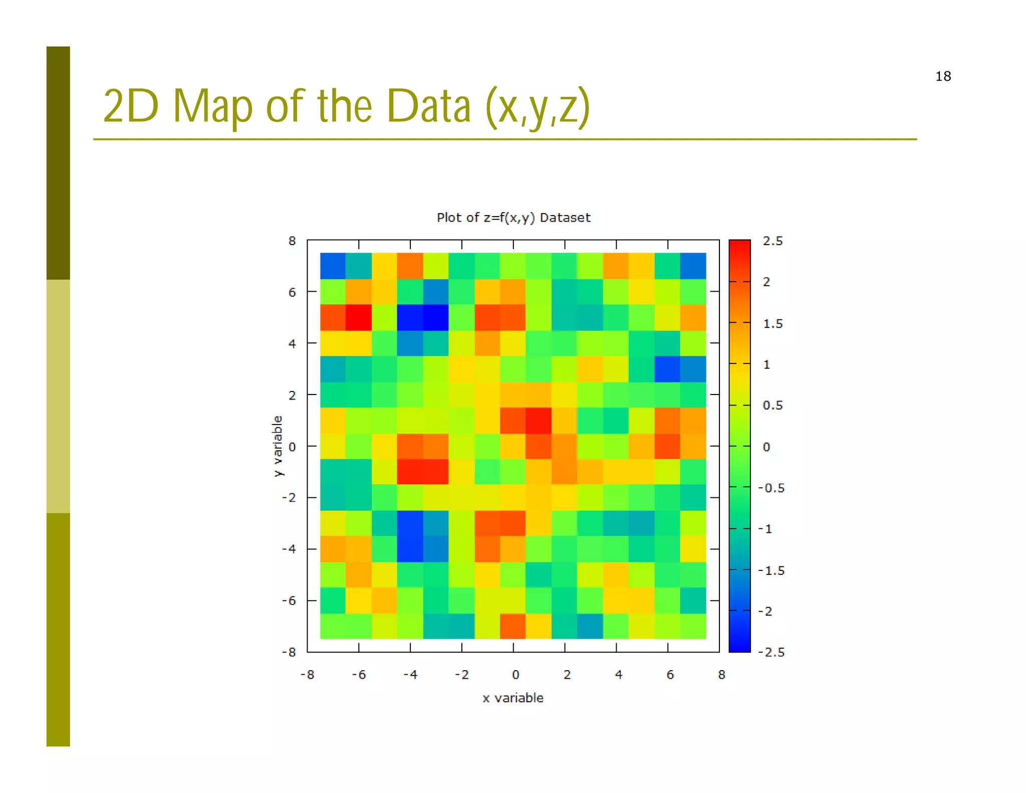
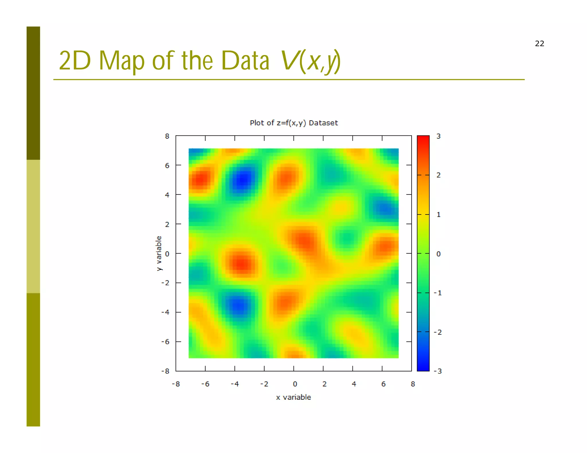
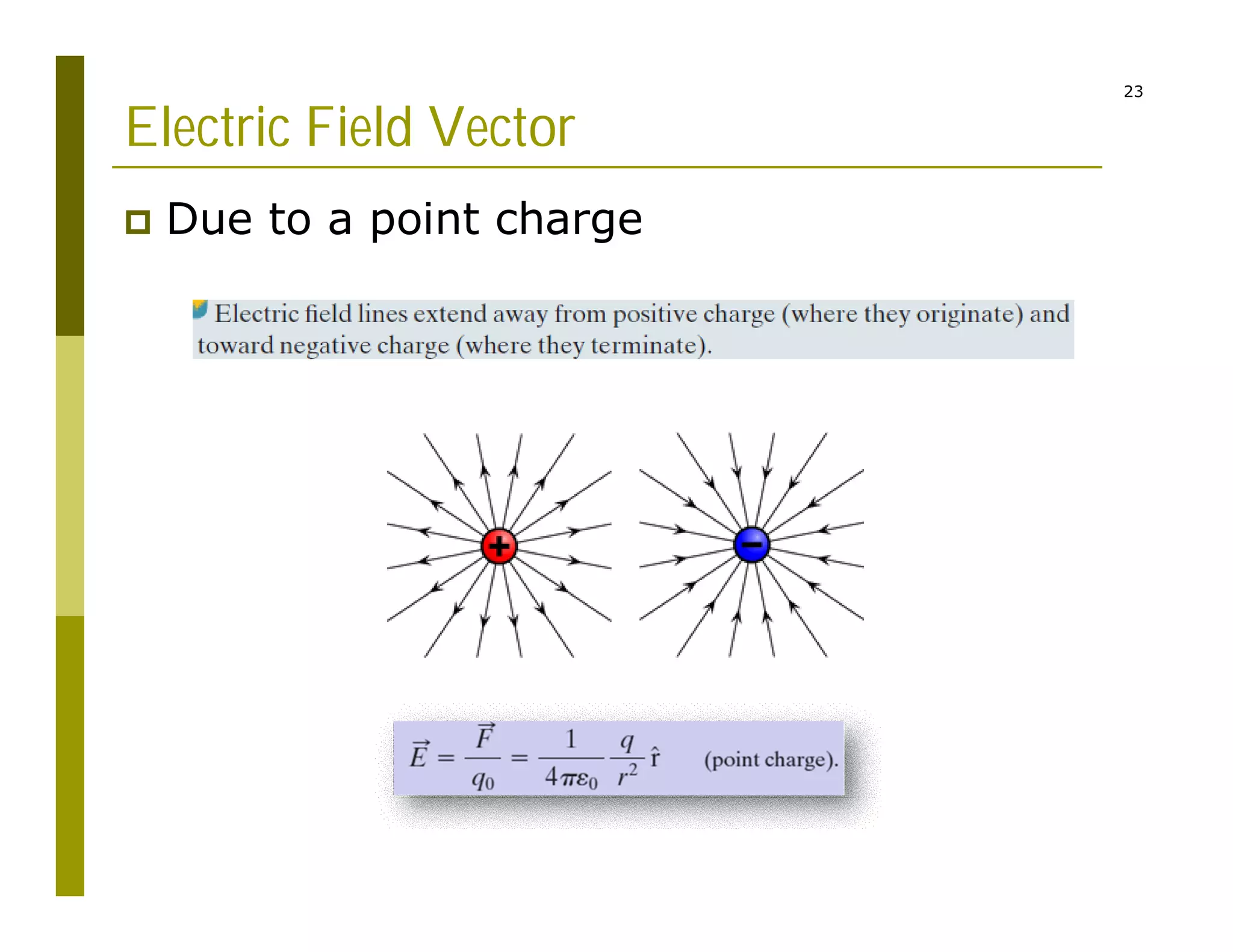
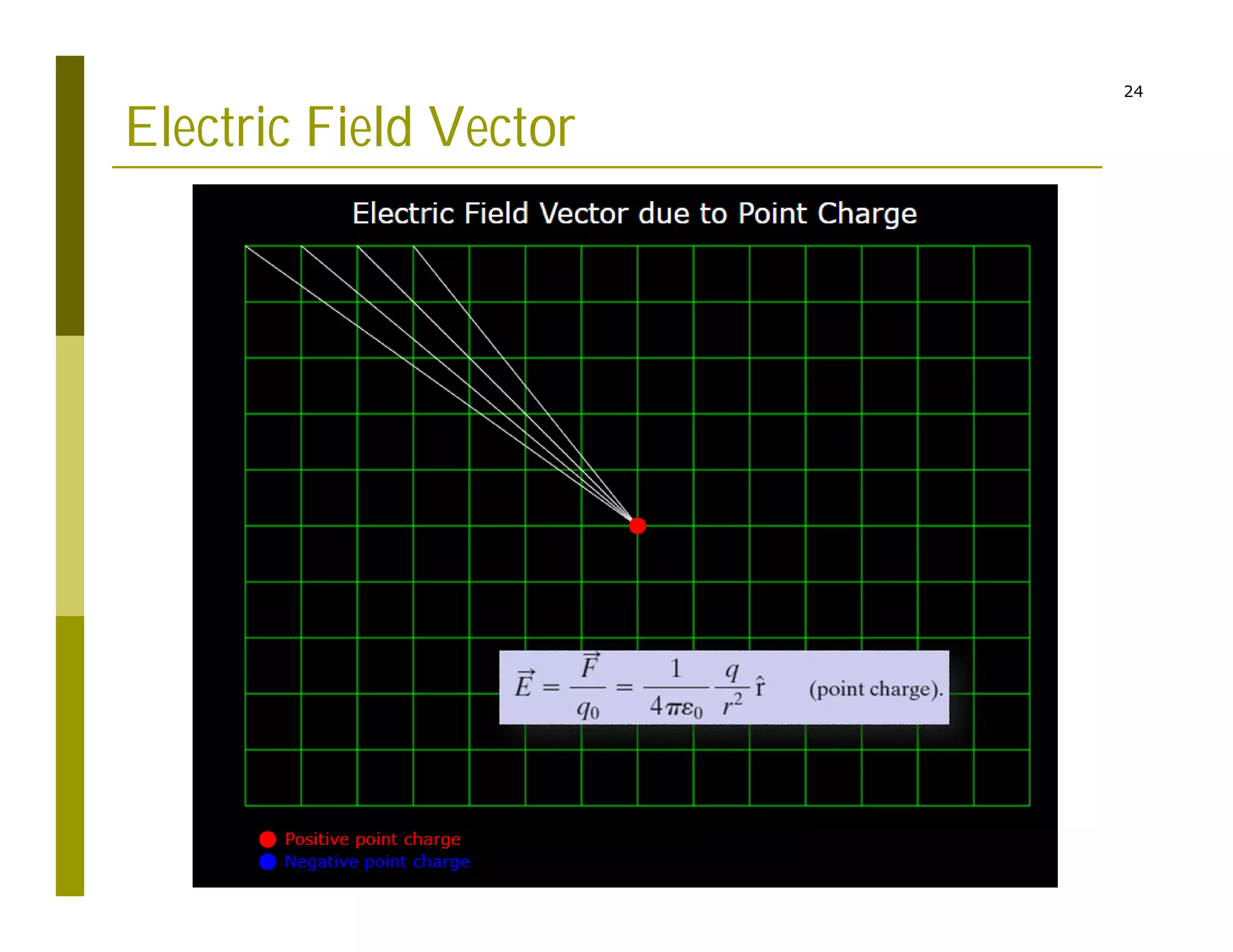
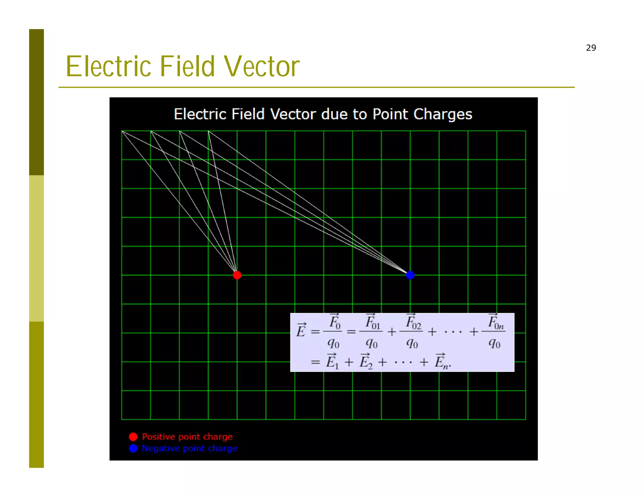
1
1
Programming, Computation, Simulation
Applications in Math & Physics
Graphical Data Representation
Syeilendra Pramuditya
Department of Physics
Institut Teknologi Bandung
2
Potential Due to a Point Charge
Consider a point P at distance R from a fixed particle of positive
charge q. Imagine that we move a positive test charge q0 from point
P to infinity. The path chosen can be the simplest one— a line that
extends radially from the fixed particle through P to infinity.
If Vf =0 (at ∞) and Vi =V (at R). Then, for the magnitude of the
electric field at the site of the test charge,
That gives:
Switching R to r,
A positively charged particle produces a positive electric potential.
A negatively charged particle produces a negative electric potential.
3
Potential Due to Point Charges:
The net potential at a point due to a group of point charges can be
found with the help of the superposition principle. First the
individual potential resulting from each charge is considered at the
given point. Then we sum the potentials.
For n charges, the net potential is
Scalar Equation (Easy)
r
4
Potential Due to Point Charges:
5
Code Structure
 Read Input (input.txt)
 How many particles?
 Charge of each particle
 Location of each particle
 Calculation domain (xmin, ymin, xmax, ymax)
 Grid resolution
6
Code Structure
 Calculate potential at all grid-points (nim.pas)
1
Use 5 and dimensionless variables
n
i
i i
q
V k
r
k




7
Code Structure
 Write Output to Datafile (output.txt)
8
Plot Output Data
 myplot.gpt
9
2D Map of the Data (x,y,z)
10
Data Interpolation
 Data xy
11
Data Interpolation
 Lagrange Interpolation
 Based on Taylor series
 General: Polynomial
 Simplest: Linear, y = ax + b
 And many more methods..
Ref.: A First Course in Computational Physics, Chapter 3, Paul DeVries
12
Lagrange Linear Interpolation
1 2 1 2
2 1 2 1
2 1 1 2 2 1 1 2
( ) ( ) ( )
x x x x x x x x
p x f x f x y y
x x x x x x x x
   
   
   
x1,y1
x2,y2
p(x)
2 1 2 4 5
( 2) 5 3 2 3.67
4 1 1 4 3
p x
 
     
 
13
Lagrange Linear Interpolation
1 2 1 2
2 1 1 2
2 1 1 2
1
( )
2 2
x x x x x x
p x y y y y
x x x x
 
  
    
 
 
 
x1,y1
x2,y2
p(x)
1 4 1
(2.5) (3 5) 4
2 2
p p

 
   
 
 
Interpolated data is
at midpoint
14
Tabular Data File (x,y,z)
Contoh file output data
15
2D Map of the Data (x,y,z)
16
2D Interpolation for Plot Smoothing
Data
Interpolated
17
Code Structure
 Read Input Data File
 Interpolate Data
 Write (File/Array) Interpolated Output Data
 Generate 2D map of the data
18
2D Map of the Data (x,y,z)
19
2D Map of the Data (x,y,z)
20
2D Map of the Data (x,y,z)
21
2D Map of the Data (x,y,z)
22
2D Map of the Data V(x,y)
23
Electric Field Vector
 Due to a point charge
24
Electric Field Vector
25
Electric Field Vector
26
Electric Field Vector
 Real magnitude of vector
27
Electric Field Vector
 Equal magnitude of vector
28
Electric Field Vector
 Multiple Charged Particles
The net, or resultant, electric field due to more than one point charge
can be found by the superposition principle. The net electric field at
the position of the test charge is
29
Electric Field Vector
30
Electric Field Vector
31
Electric Field Vector
 Real magnitude of vector
32
Electric Field Vector
 Equal magnitude of vector
33
Code Structure
 Read Input
 How many particles?
 Location of each particle
 Charge of each particle
 Calculation domain (xmin, ymin, xmax, ymax)
 Grid resolution
 Calculate electric field vector at all nodes/grid-
points
 Write Output to Datafile (depends on your
graphic tools)
 Position, magnitude, angle
 x1, y1, x2, y2
 Generate vector map of the output data

SPSF02 - Graphical Data Representation