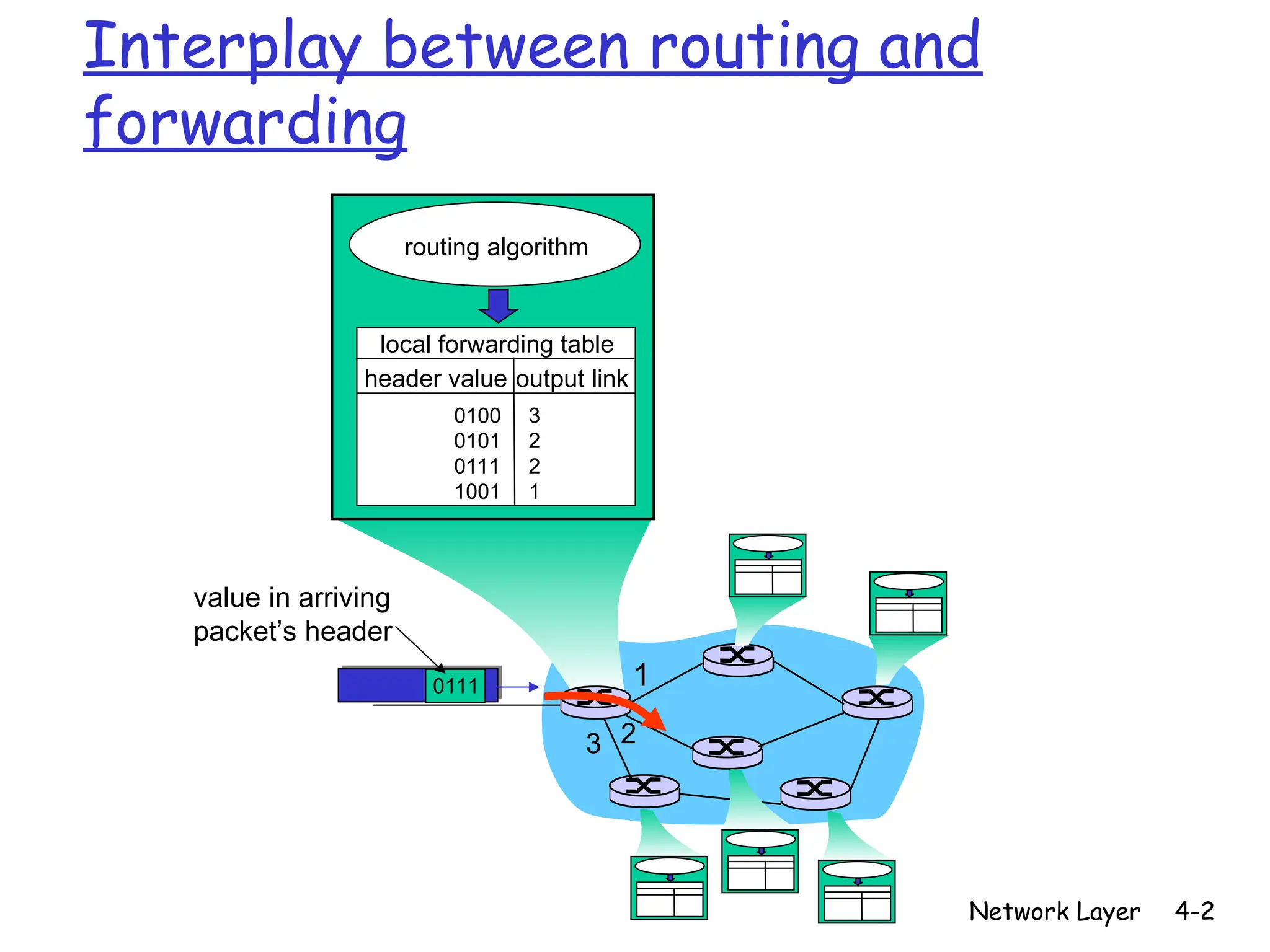
Network Layer 4-2
1
2
3
0111
valuein arriving
packet’s header
routing algorithm
local forwarding table
header value output link
0100
0101
0111
1001
3
2
2
1
Interplay between routing and
forwarding
3.
Network Layer 4-3
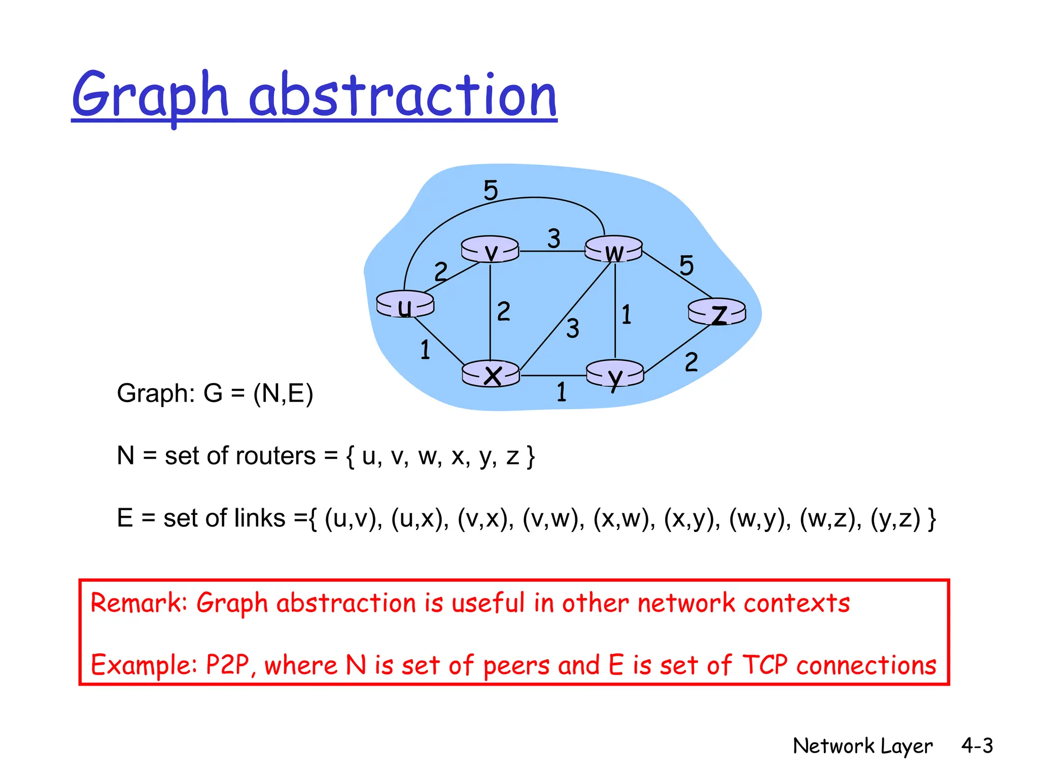
u
y
x
w
v
z
2
2
1
3
1
1
2
5
3
5
Graph:G = (N,E)
N = set of routers = { u, v, w, x, y, z }
E = set of links ={ (u,v), (u,x), (v,x), (v,w), (x,w), (x,y), (w,y), (w,z), (y,z) }
Graph abstraction
Remark: Graph abstraction is useful in other network contexts
Example: P2P, where N is set of peers and E is set of TCP connections
4.
Network Layer 4-4
Graphabstraction: costs
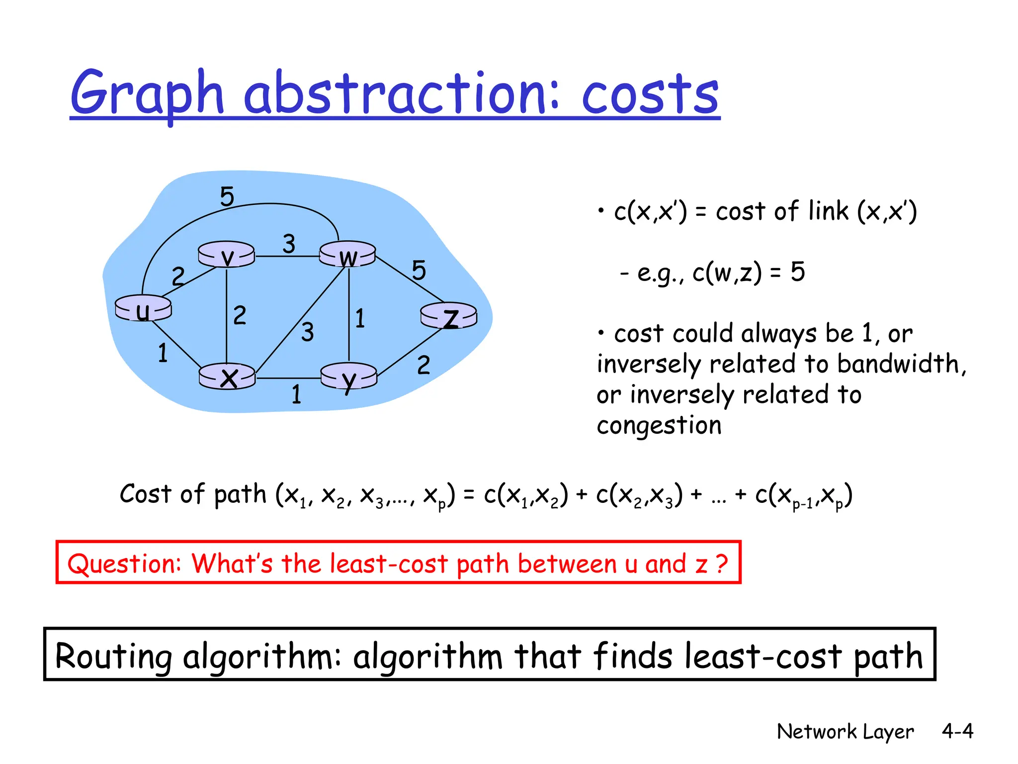
u
y
x
w
v
z
2
2
1
3
1
1
2
5
3
5
• c(x,x’) = cost of link (x,x’)
- e.g., c(w,z) = 5
• cost could always be 1, or
inversely related to bandwidth,
or inversely related to
congestion
Cost of path (x1, x2, x3,…, xp) = c(x1,x2) + c(x2,x3) + … + c(xp-1,xp)
Question: What’s the least-cost path between u and z ?
Routing algorithm: algorithm that finds least-cost path
5.
Network Layer 4-5
RoutingAlgorithm classification
Global or decentralized
information?
Global:
all routers have complete
topology, link cost info
“link state” algorithms
Decentralized:
router knows physically-
connected neighbors, link costs
to neighbors
iterative process of
computation, exchange of info
with neighbors
“distance vector” algorithms
Static or dynamic?
Static:
routes change slowly over
time
Dynamic:
routes change more quickly
periodic update
in response to link cost
changes
6.
Network Layer 4-6
ALink-State Routing Algorithm
Dijkstra’s algorithm
net topology, link costs known
to all nodes
accomplished via “link
state broadcast”
all nodes have same info
computes least cost paths
from one node (‘source”) to all
other nodes
gives forwarding table for
that node
iterative: after k iterations,
know least cost path to k
dest.’s
Notation:
c(x,y): link cost from node x
to y; = ∞ if not direct
neighbors
D(v): current value of cost of
path from source to dest. v
p(v): predecessor node along
path from source to v
N': set of nodes whose least
cost path definitively known
7.
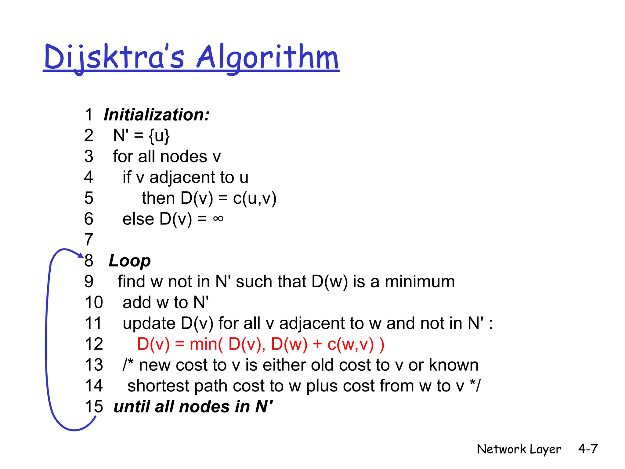
Network Layer 4-7
Dijsktra’sAlgorithm
1 Initialization:
2 N' = {u}
3 for all nodes v
4 if v adjacent to u
5 then D(v) = c(u,v)
6 else D(v) = ∞
7
8 Loop
9 find w not in N' such that D(w) is a minimum
10 add w to N'
11 update D(v) for all v adjacent to w and not in N' :
12 D(v) = min( D(v), D(w) + c(w,v) )
13 /* new cost to v is either old cost to v or known
14 shortest path cost to w plus cost from w to v */
15 until all nodes in N'
8.
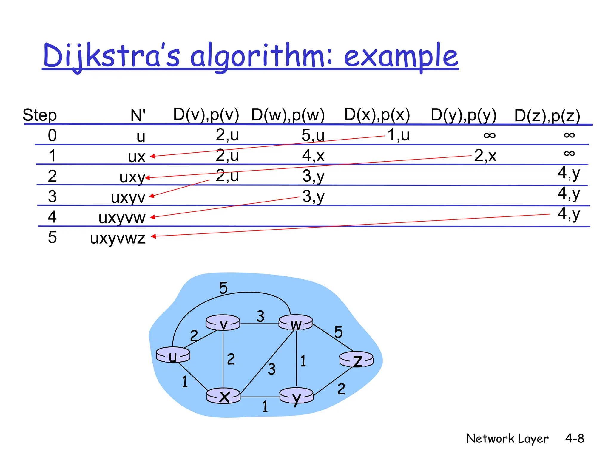
Network Layer 4-8
Dijkstra’salgorithm: example
Step
0
1
2
3
4
5
N'
u
ux
uxy
uxyv
uxyvw
uxyvwz
D(v),p(v)
2,u
2,u
2,u
D(w),p(w)
5,u
4,x
3,y
3,y
D(x),p(x)
1,u
D(y),p(y)
∞
2,x
D(z),p(z)
∞
∞
4,y
4,y
4,y
u
y
x
w
v
z
2
2
1
3
1
1
2
5
3
5
9.
Network Layer 4-9
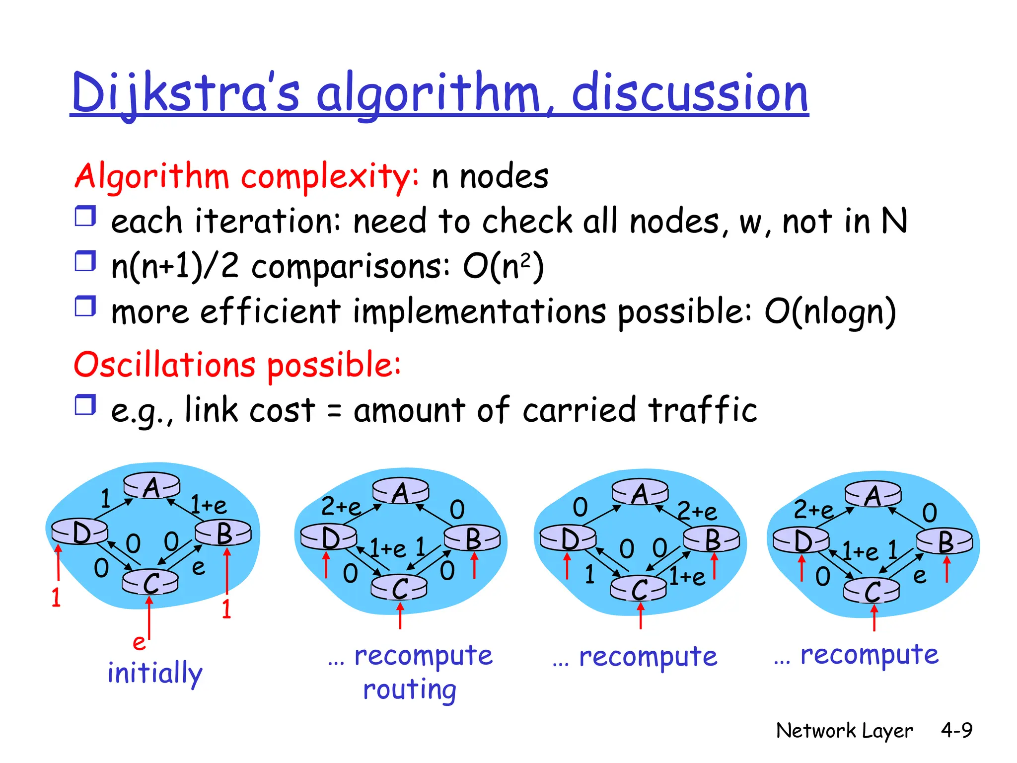
Dijkstra’salgorithm, discussion
Algorithm complexity: n nodes
each iteration: need to check all nodes, w, not in N
n(n+1)/2 comparisons: O(n2
)
more efficient implementations possible: O(nlogn)
Oscillations possible:
e.g., link cost = amount of carried traffic
A
D
C
B
1 1+e
e
0
e
1 1
0 0
A
D
C
B
2+e 0
0
0
1+e 1
A
D
C
B
0 2+e
1+e
1
0 0
A
D
C
B
2+e 0
e
0
1+e 1
initially
… recompute
routing
… recompute … recompute
10.
Network Layer 4-10
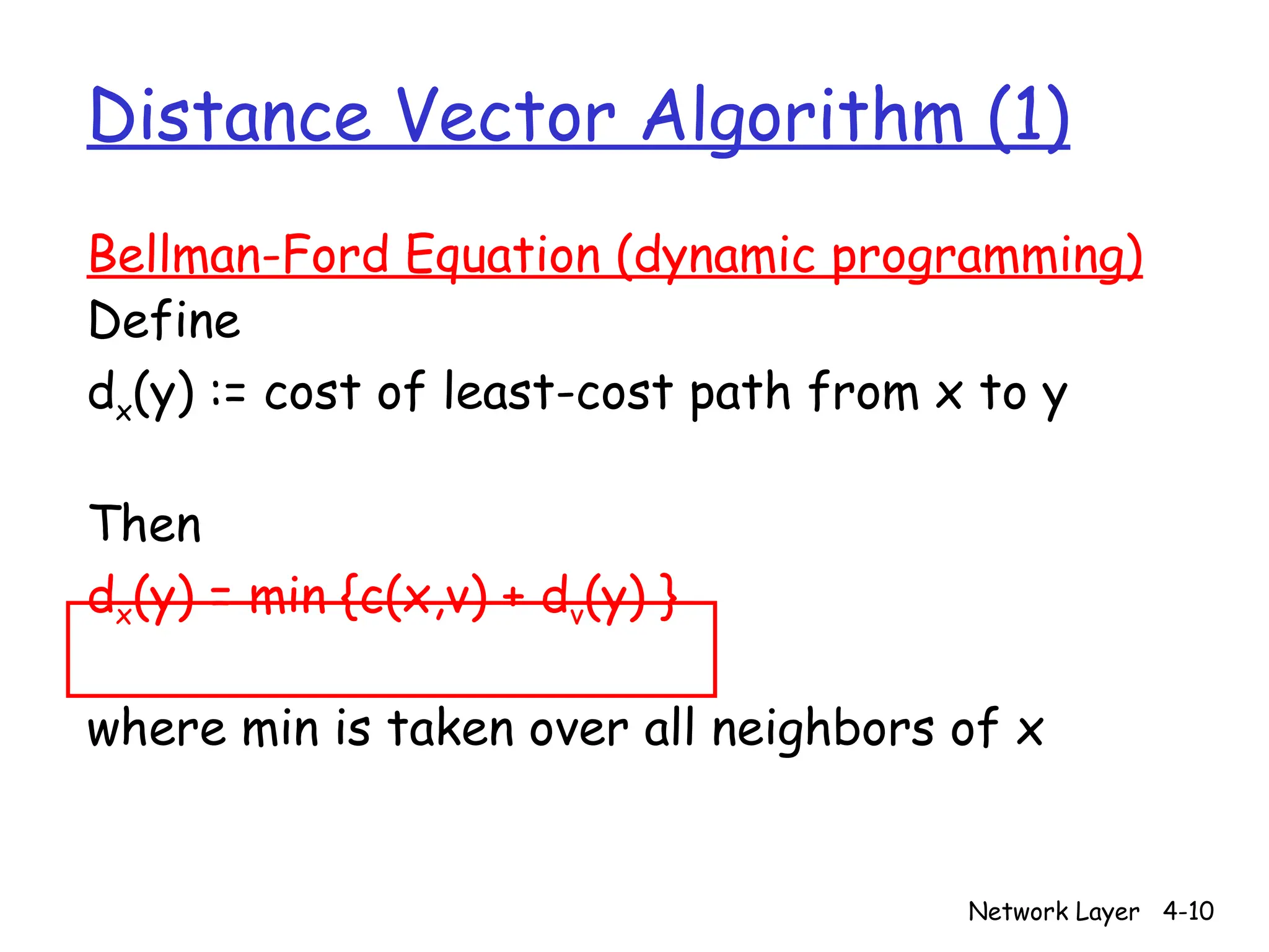
DistanceVector Algorithm (1)
Bellman-Ford Equation (dynamic programming)
Define
dx(y) := cost of least-cost path from x to y
Then
dx(y) = min {c(x,v) + dv(y) }
where min is taken over all neighbors of x
11.
Network Layer 4-11
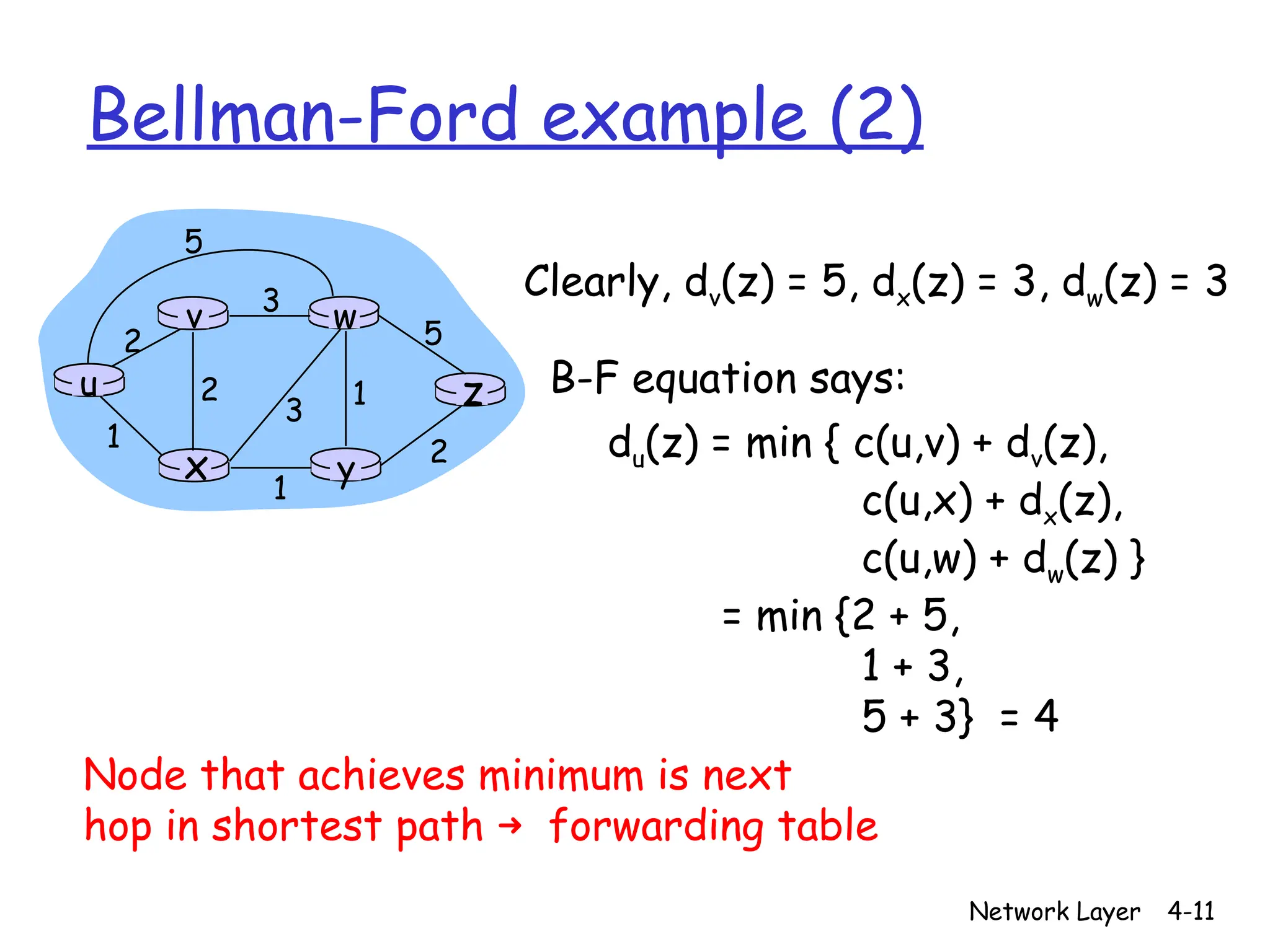
Bellman-Fordexample (2)
u
y
x
w
v
z
2
2
1
3
1
1
2
5
3
5
Clearly, dv(z) = 5, dx(z) = 3, dw(z) = 3
du(z) = min { c(u,v) + dv(z),
c(u,x) + dx(z),
c(u,w) + dw(z) }
= min {2 + 5,
1 + 3,
5 + 3} = 4
Node that achieves minimum is next
hop in shortest path ➜ forwarding table
B-F equation says:
12.
Network Layer 4-12
DistanceVector Algorithm (3)
Dx(y) = estimate of least cost from x to y
Distance vector: Dx = [Dx(y): y є N ]
Node x knows cost to each neighbor v:
c(x,v)
Node x maintains Dx = [Dx(y): y є N ]
Node x also maintains its neighbors’
distance vectors
For each neighbor v, x maintains
Dv = [Dv(y): y є N ]
13.
Network Layer 4-13
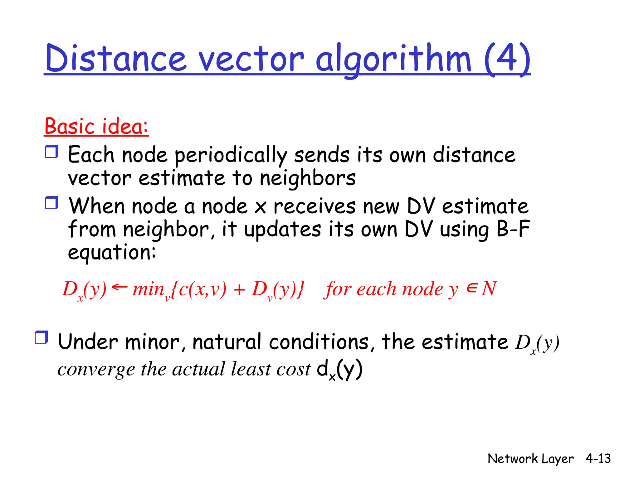
Distancevector algorithm (4)
Basic idea:
Each node periodically sends its own distance
vector estimate to neighbors
When node a node x receives new DV estimate
from neighbor, it updates its own DV using B-F
equation:
Dx
(y) ← minv
{c(x,v) + Dv
(y)} for each node y ∊ N
Under minor, natural conditions, the estimate Dx
(y)
converge the actual least cost dx(y)
14.
Network Layer 4-14
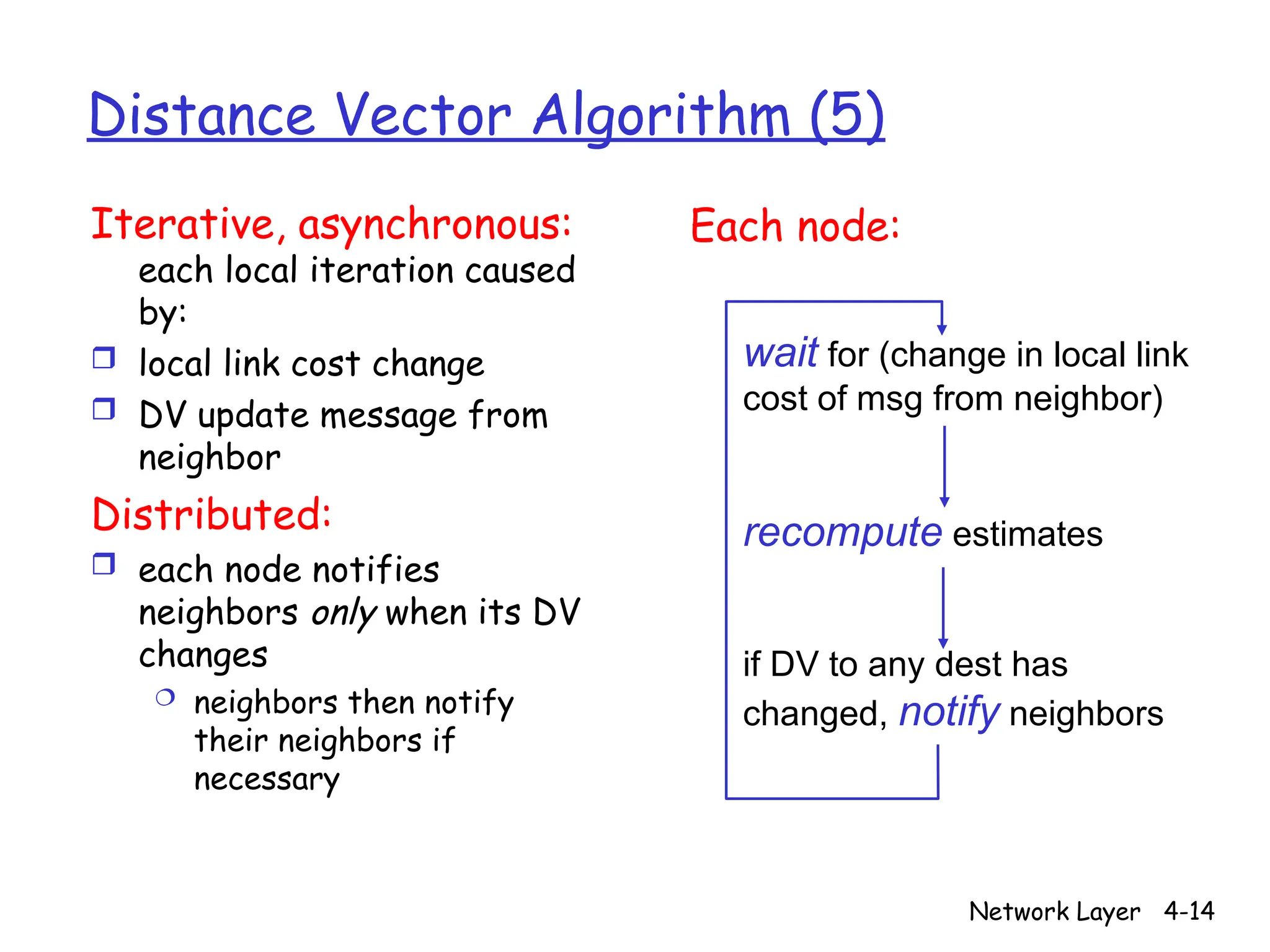
DistanceVector Algorithm (5)
Iterative, asynchronous:
each local iteration caused
by:
local link cost change
DV update message from
neighbor
Distributed:
each node notifies
neighbors only when its DV
changes
neighbors then notify
their neighbors if
necessary
wait for (change in local link
cost of msg from neighbor)
recompute estimates
if DV to any dest has
changed, notify neighbors
Each node:
15.
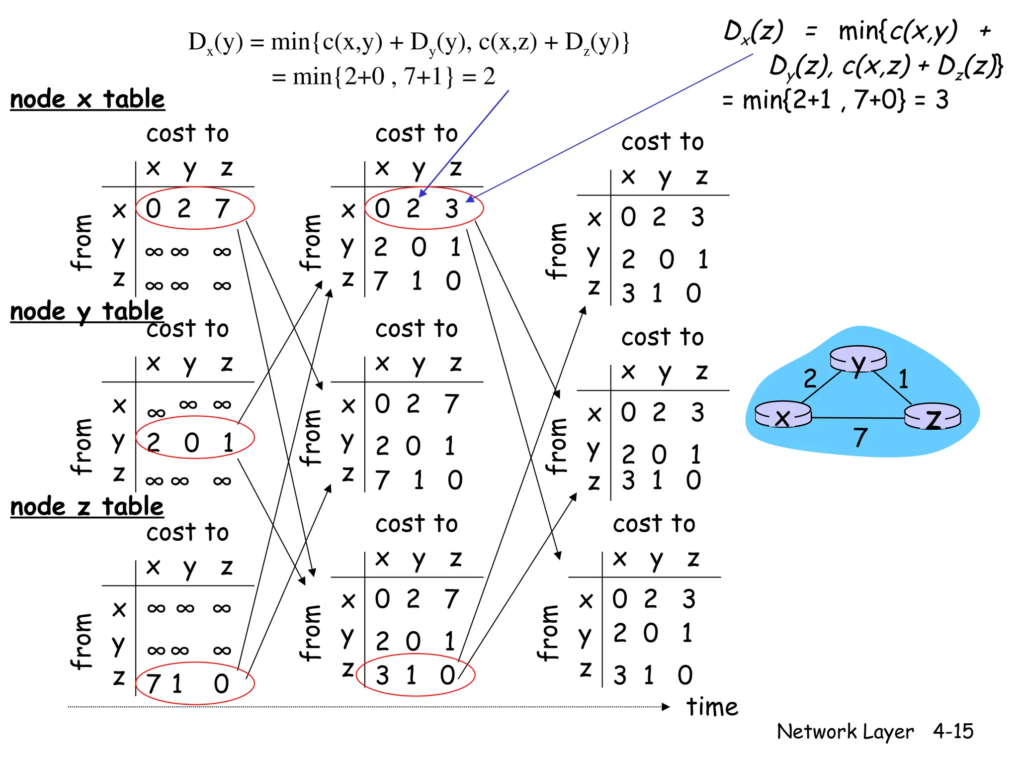
Network Layer 4-15
xy z
x
y
z
0 2 7
∞ ∞ ∞
∞ ∞ ∞
from
cost to
from
from
x y z
x
y
z
0 2 3
from
cost to
x y z
x
y
z
0 2 3
from
cost to
x y z
x
y
z
∞ ∞
∞ ∞ ∞
cost to
x y z
x
y
z
0 2 7
from
cost to
x y z
x
y
z
0 2 3
from
cost to
x y z
x
y
z
0 2 3
from
cost to
x y z
x
y
z
0 2 7
from
cost to
x y z
x
y
z
∞∞ ∞
7 1 0
cost to
∞
2 0 1
∞ ∞ ∞
2 0 1
7 1 0
2 0 1
7 1 0
2 0 1
3 1 0
2 0 1
3 1 0
2 0 1
3 1 0
2 0 1
3 1 0
time
x z
1
2
7
y
node x table
node y table
node z table
Dx(y) = min{c(x,y) + Dy(y), c(x,z) + Dz(y)}
= min{2+0 , 7+1} = 2
Dx(z) = min{c(x,y) +
Dy(z), c(x,z) + Dz(z)}
= min{2+1 , 7+0} = 3
16.
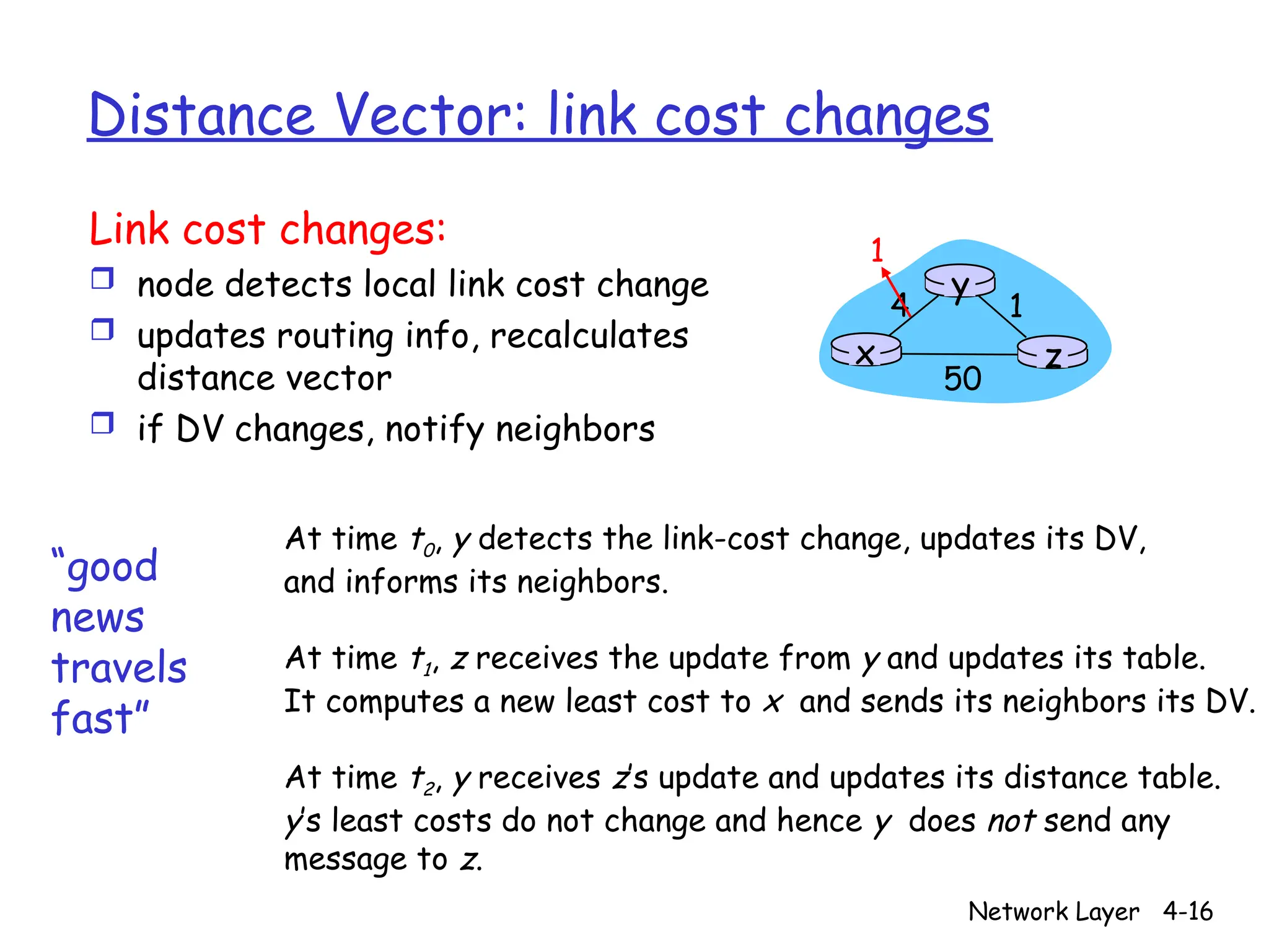
Network Layer 4-16
DistanceVector: link cost changes
Link cost changes:
node detects local link cost change
updates routing info, recalculates
distance vector
if DV changes, notify neighbors
“good
news
travels
fast”
x z
1
4
50
y
1
At time t0, y detects the link-cost change, updates its DV,
and informs its neighbors.
At time t1, z receives the update from y and updates its table.
It computes a new least cost to x and sends its neighbors its DV.
At time t2, y receives z’s update and updates its distance table.
y’s least costs do not change and hence y does not send any
message to z.
17.
Network Layer 4-17
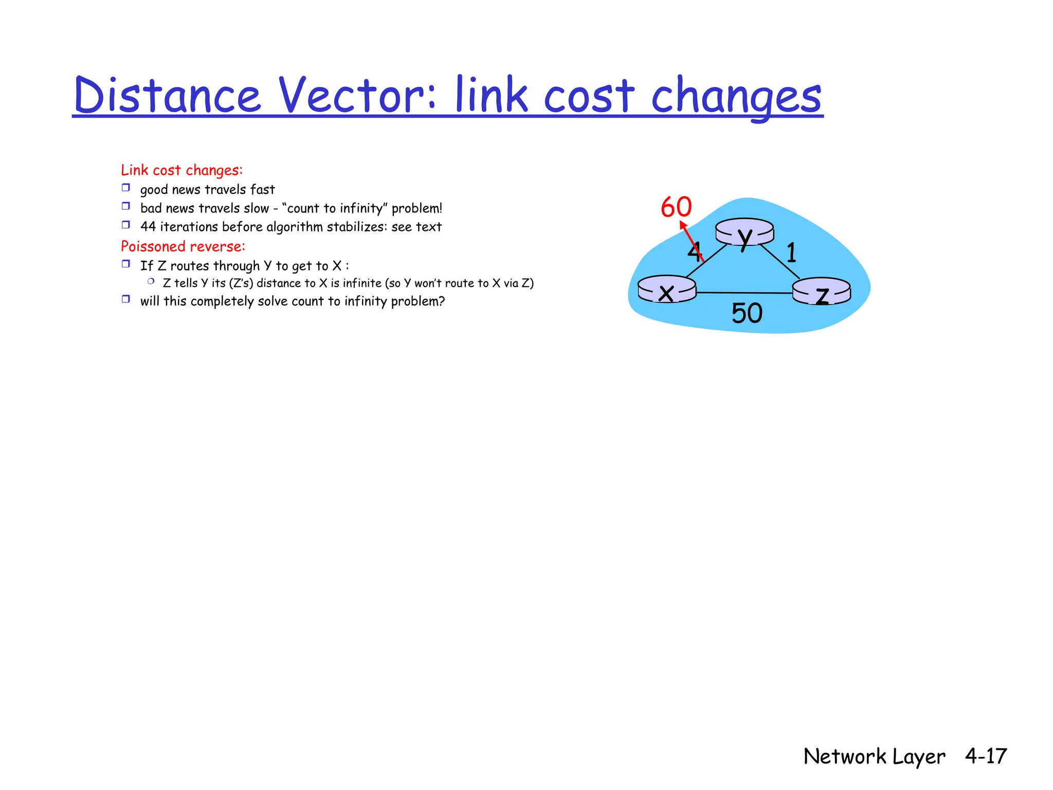
DistanceVector: link cost changes
Link cost changes:
good news travels fast
bad news travels slow - “count to infinity” problem!
44 iterations before algorithm stabilizes: see text
Poissoned reverse:
If Z routes through Y to get to X :
Z tells Y its (Z’s) distance to X is infinite (so Y won’t route to X via Z)
will this completely solve count to infinity problem? x z
1
4
50
y
60
18.
Network Layer 4-18
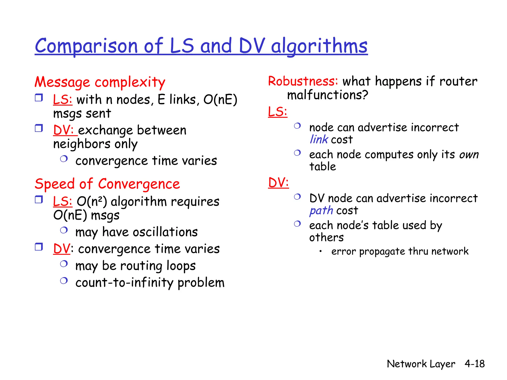
Comparisonof LS and DV algorithms
Message complexity
LS: with n nodes, E links, O(nE)
msgs sent
DV: exchange between
neighbors only
convergence time varies
Speed of Convergence
LS: O(n2
) algorithm requires
O(nE) msgs
may have oscillations
DV: convergence time varies
may be routing loops
count-to-infinity problem
Robustness: what happens if router
malfunctions?
LS:
node can advertise incorrect
link cost
each node computes only its own
table
DV:
DV node can advertise incorrect
path cost
each node’s table used by
others
• error propagate thru network
19.
Network Layer 4-19
HierarchicalRouting
scale: with 200 million
destinations:
can’t store all dest’s in
routing tables!
routing table exchange
would swamp links!
administrative autonomy
internet = network of
networks
each network admin may
want to control routing in its
own network
Our routing study thus far - idealization
all routers identical
network “flat”
… not true in practice
20.
Network Layer 4-20
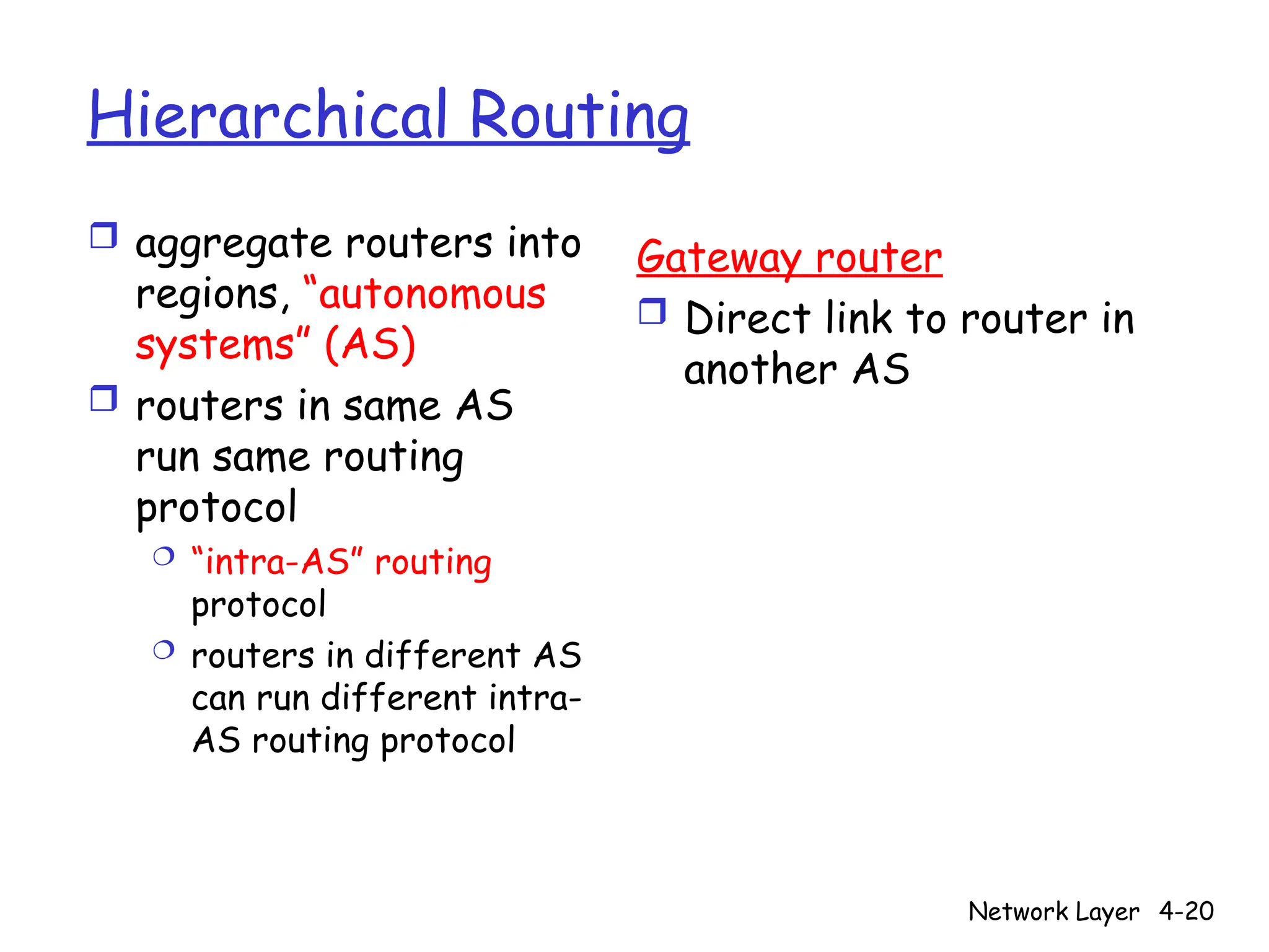
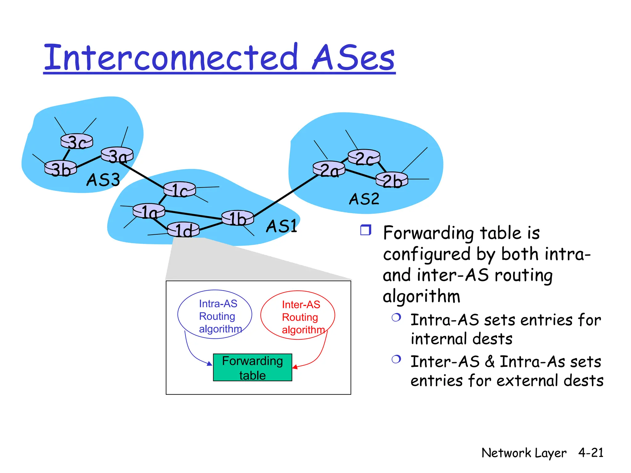
HierarchicalRouting
aggregate routers into
regions, “autonomous
systems” (AS)
routers in same AS
run same routing
protocol
“intra-AS” routing
protocol
routers in different AS
can run different intra-
AS routing protocol
Gateway router
Direct link to router in
another AS
Network Layer 4-22
3b
1d
3a
1c
2a
AS3
AS1
AS2
1a
2c
2b
1b
3c
Inter-AStasks
Suppose router in AS1
receives datagram for
which dest is outside
of AS1
Router should forward
packet towards on of
the gateway routers,
but which one?
AS1 needs:
1. to learn which dests
are reachable through
AS2 and which
through AS3
2. to propagate this
reachability info to all
routers in AS1
Job of inter-AS routing!
23.
Network Layer 4-23
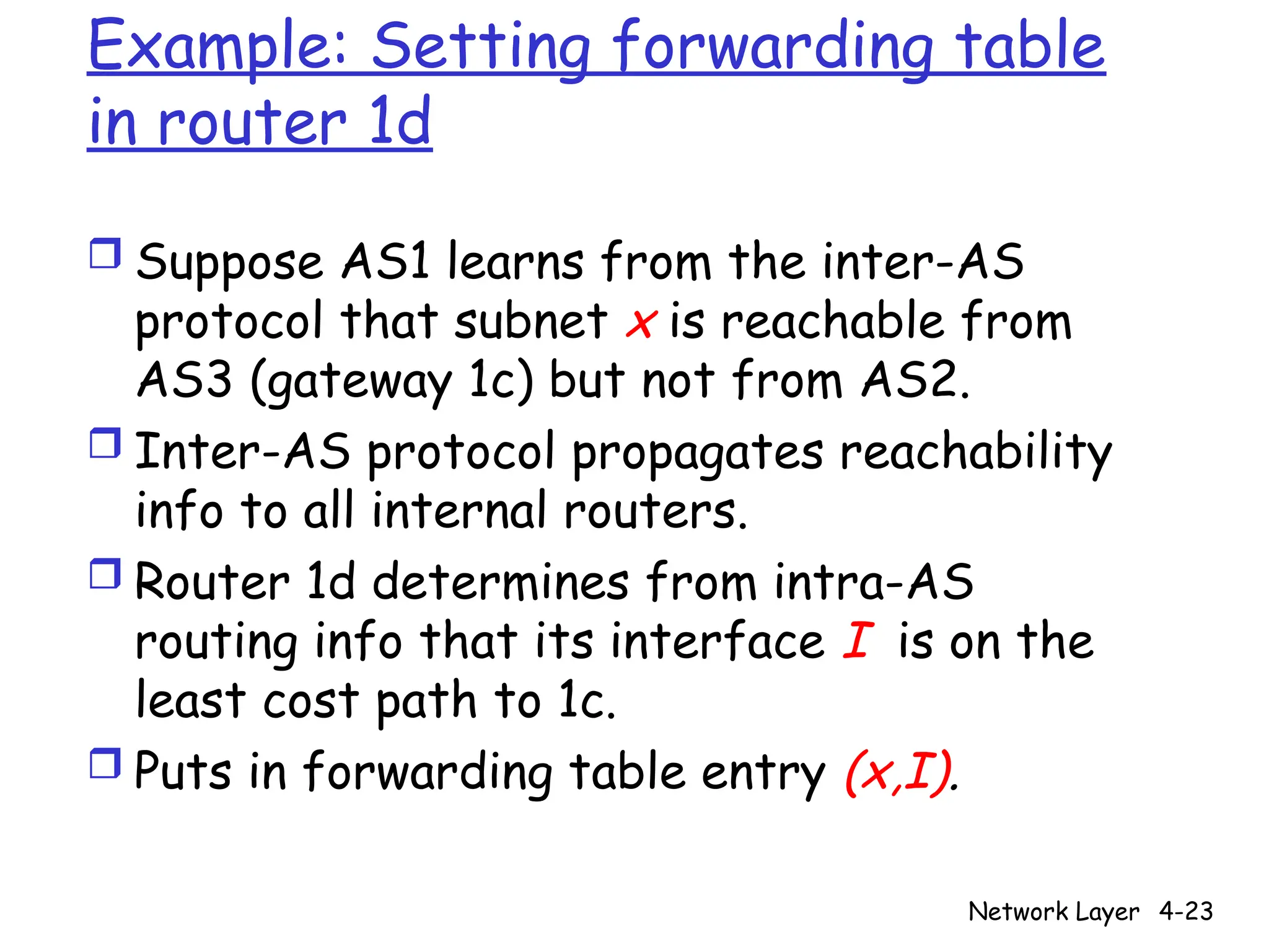
Example:Setting forwarding table
in router 1d
Suppose AS1 learns from the inter-AS
protocol that subnet x is reachable from
AS3 (gateway 1c) but not from AS2.
Inter-AS protocol propagates reachability
info to all internal routers.
Router 1d determines from intra-AS
routing info that its interface I is on the
least cost path to 1c.
Puts in forwarding table entry (x,I).
24.
Network Layer 4-24
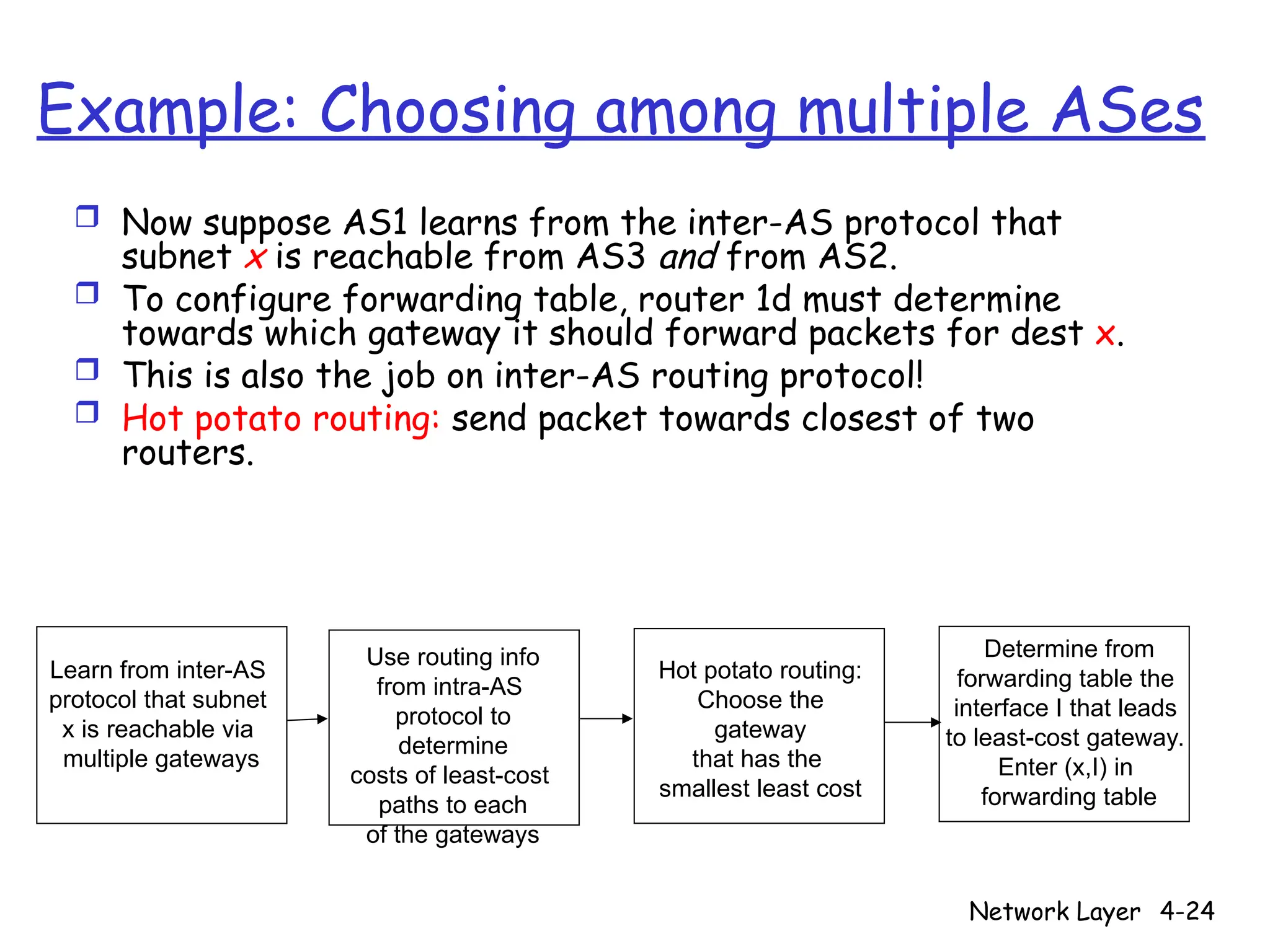
Learnfrom inter-AS
protocol that subnet
x is reachable via
multiple gateways
Use routing info
from intra-AS
protocol to
determine
costs of least-cost
paths to each
of the gateways
Hot potato routing:
Choose the
gateway
that has the
smallest least cost
Determine from
forwarding table the
interface I that leads
to least-cost gateway.
Enter (x,I) in
forwarding table
Example: Choosing among multiple ASes
Now suppose AS1 learns from the inter-AS protocol that
subnet x is reachable from AS3 and from AS2.
To configure forwarding table, router 1d must determine
towards which gateway it should forward packets for dest x.
This is also the job on inter-AS routing protocol!
Hot potato routing: send packet towards closest of two
routers.
25.
Network Layer 4-25
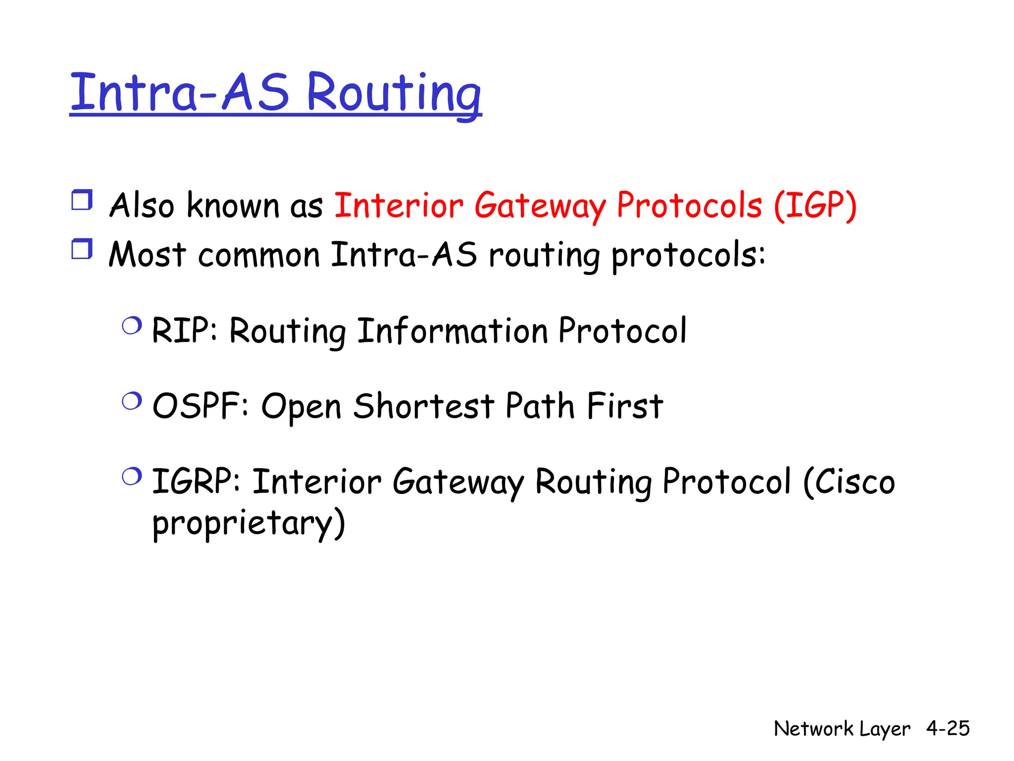
Intra-ASRouting
Also known as Interior Gateway Protocols (IGP)
Most common Intra-AS routing protocols:
RIP: Routing Information Protocol
OSPF: Open Shortest Path First
IGRP: Interior Gateway Routing Protocol (Cisco
proprietary)
26.
Network Layer 4-26
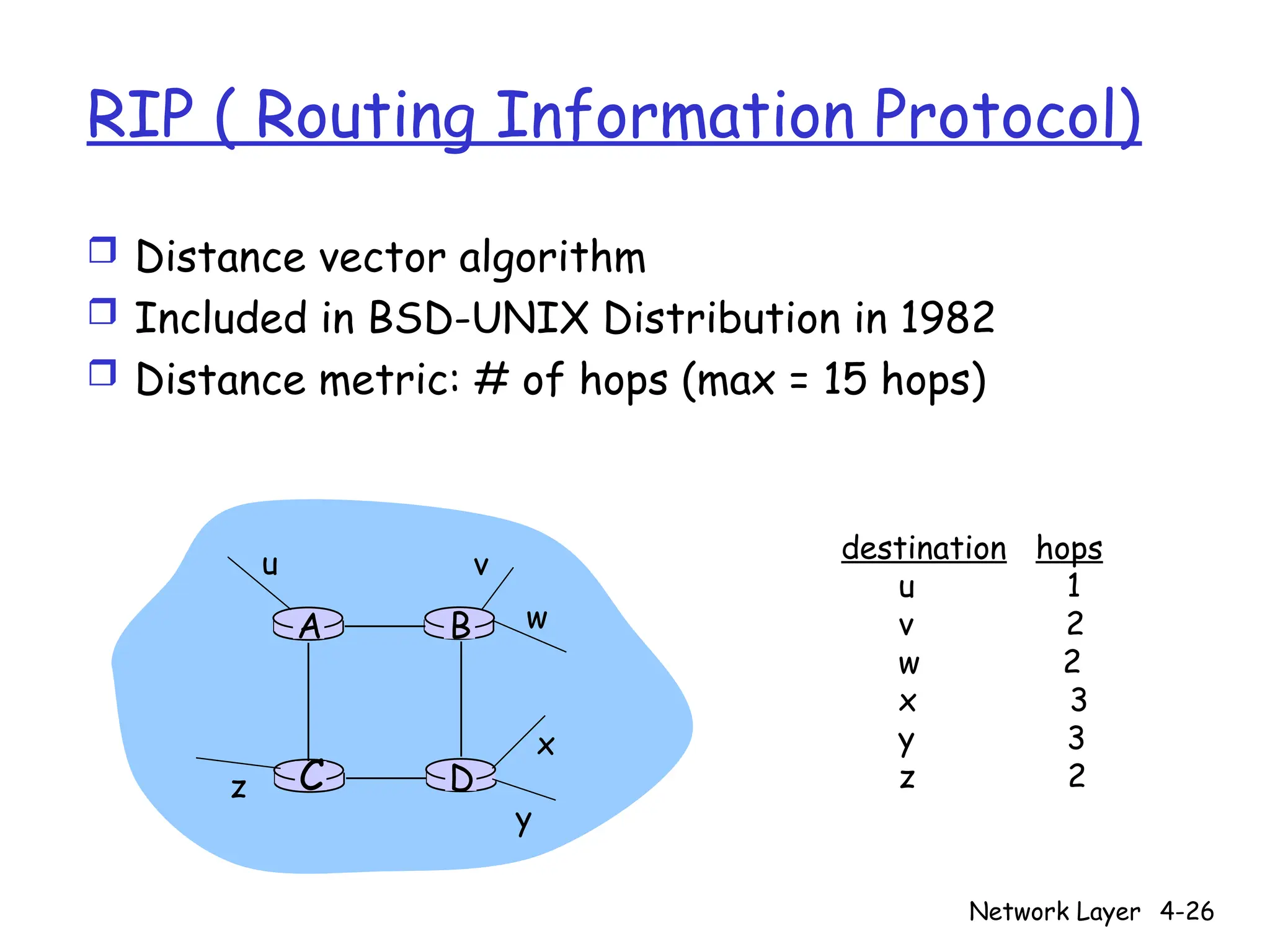
RIP( Routing Information Protocol)
Distance vector algorithm
Included in BSD-UNIX Distribution in 1982
Distance metric: # of hops (max = 15 hops)
D
C
B
A
u v
w
x
y
z
destination hops
u 1
v 2
w 2
x 3
y 3
z 2
27.
Network Layer 4-27
RIPadvertisements
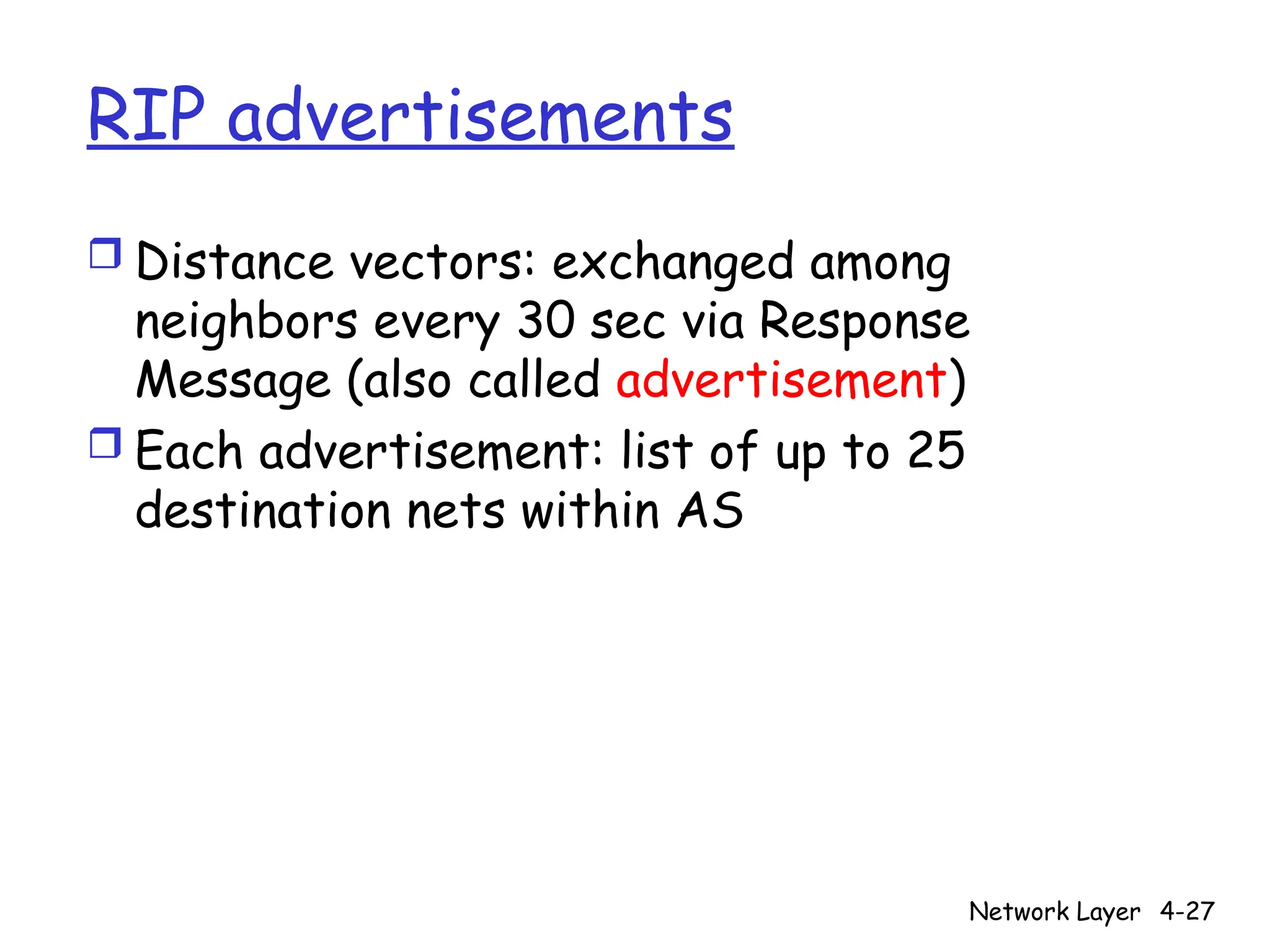
Distance vectors: exchanged among
neighbors every 30 sec via Response
Message (also called advertisement)
Each advertisement: list of up to 25
destination nets within AS
28.
Network Layer 4-28
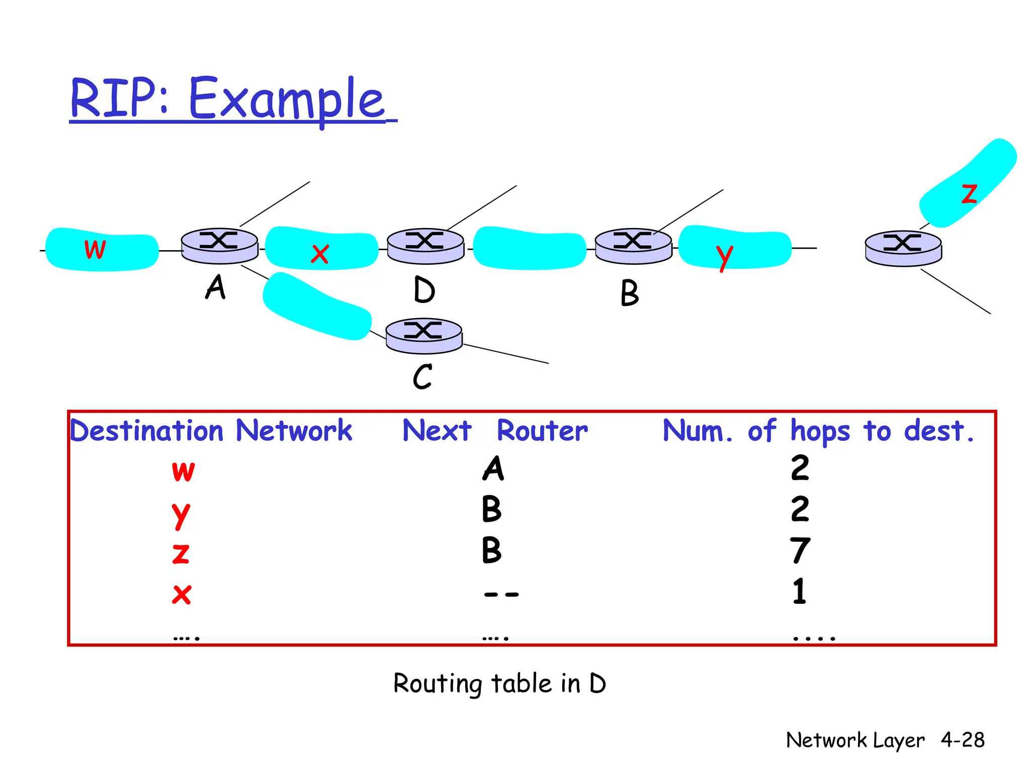
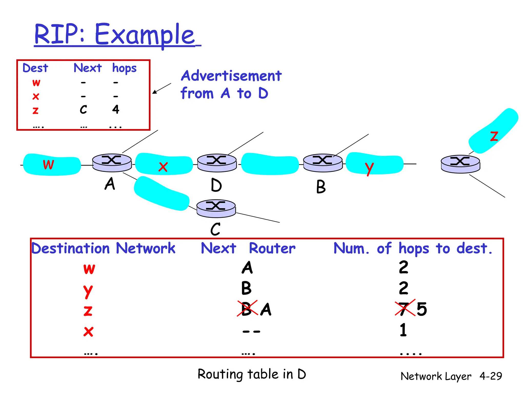
RIP:Example
Destination Network Next Router Num. of hops to dest.
w A 2
y B 2
z B 7
x -- 1
…. …. ....
w x y
z
A
C
D B
Routing table in D
29.
Network Layer 4-29
RIP:Example
Destination Network Next Router Num. of hops to dest.
w A 2
y B 2
z B A 7 5
x -- 1
…. …. ....
Routing table in D
w x y
z
A
C
D B
Dest Next hops
w - -
x - -
z C 4
…. … ...
Advertisement
from A to D
30.
Network Layer 4-30
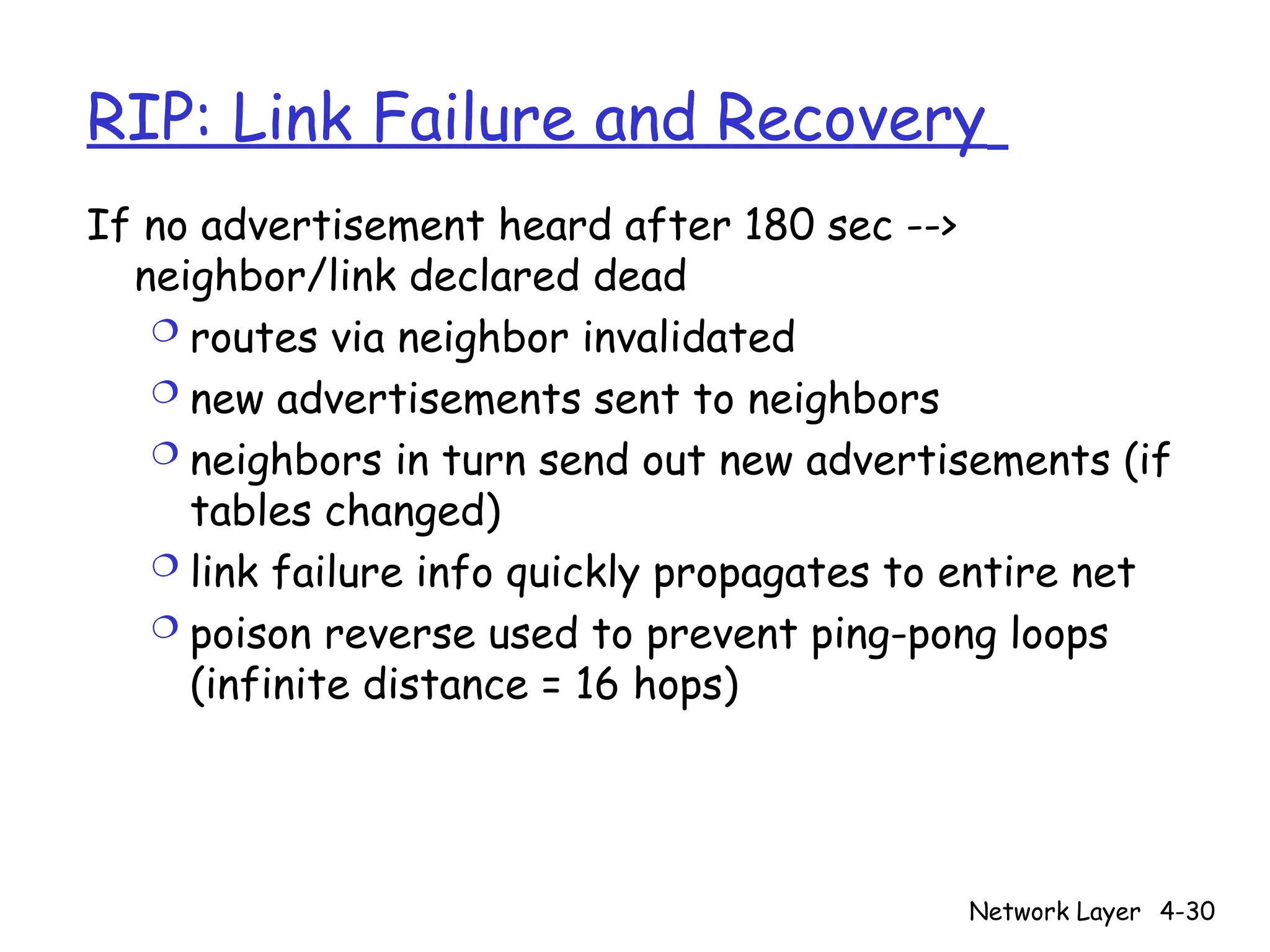
RIP:Link Failure and Recovery
If no advertisement heard after 180 sec -->
neighbor/link declared dead
routes via neighbor invalidated
new advertisements sent to neighbors
neighbors in turn send out new advertisements (if
tables changed)
link failure info quickly propagates to entire net
poison reverse used to prevent ping-pong loops
(infinite distance = 16 hops)
31.
Network Layer 4-31
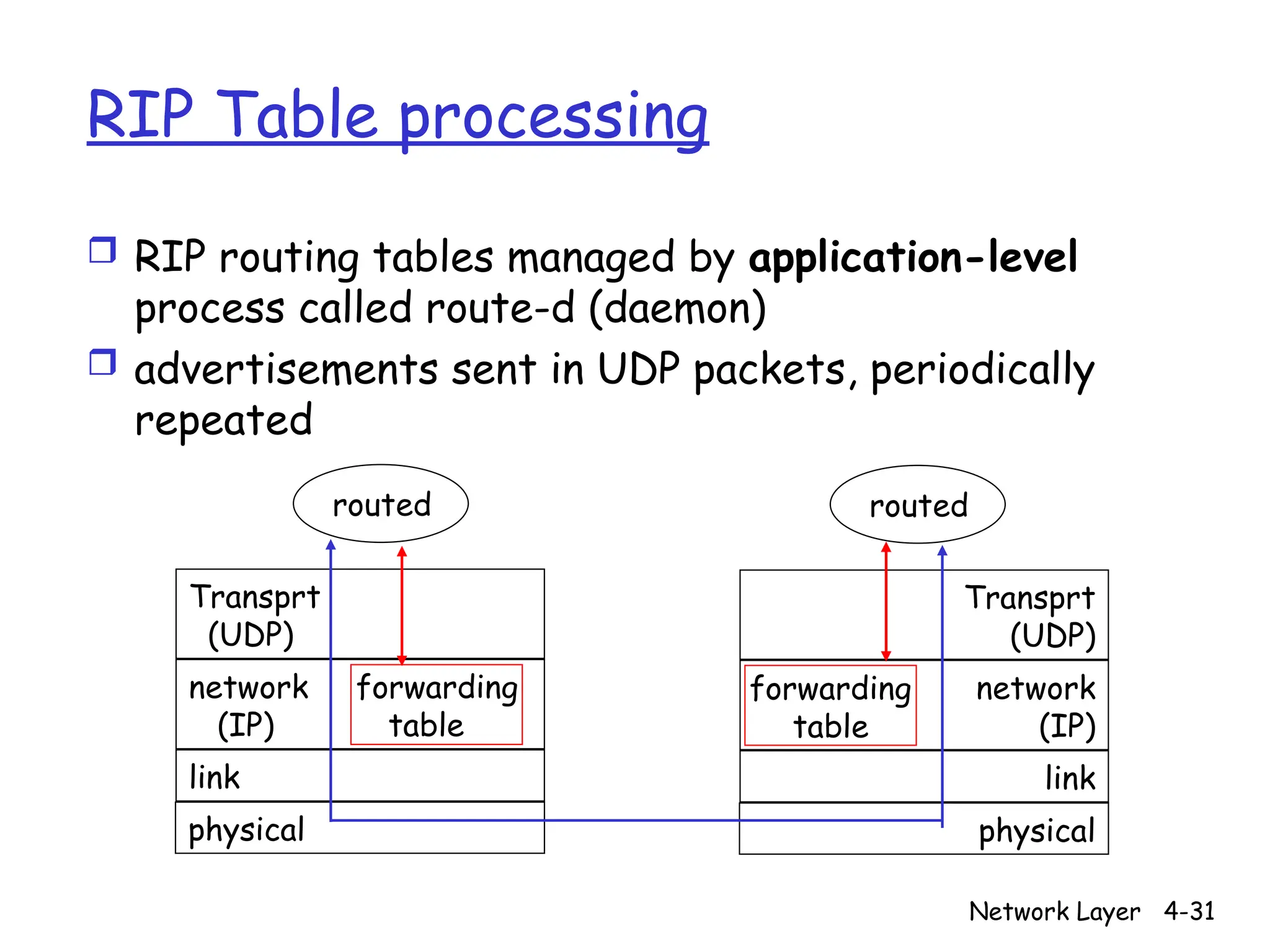
RIPTable processing
RIP routing tables managed by application-level
process called route-d (daemon)
advertisements sent in UDP packets, periodically
repeated
physical
link
network forwarding
(IP) table
Transprt
(UDP)
routed
physical
link
network
(IP)
Transprt
(UDP)
routed
forwarding
table
32.
Network Layer 4-32
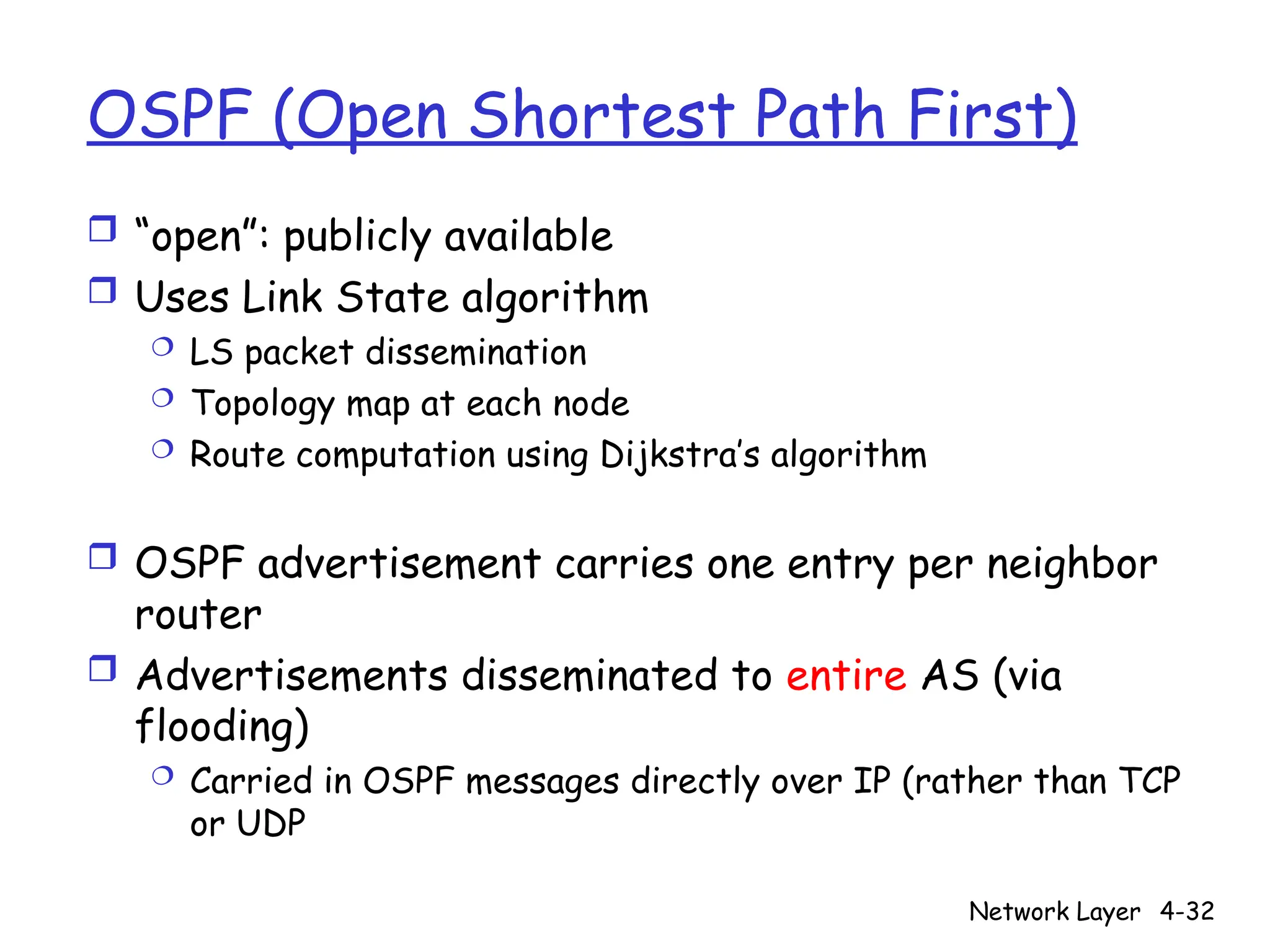
OSPF(Open Shortest Path First)
“open”: publicly available
Uses Link State algorithm
LS packet dissemination
Topology map at each node
Route computation using Dijkstra’s algorithm
OSPF advertisement carries one entry per neighbor
router
Advertisements disseminated to entire AS (via
flooding)
Carried in OSPF messages directly over IP (rather than TCP
or UDP
33.
Network Layer 4-33
OSPF“advanced” features (not in RIP)
Security: all OSPF messages authenticated (to
prevent malicious intrusion)
Multiple same-cost paths allowed (only one path in
RIP)
For each link, multiple cost metrics for different
TOS (e.g., satellite link cost set “low” for best
effort; high for real time)
Integrated uni- and multicast support:
Multicast OSPF (MOSPF) uses same topology data
base as OSPF
Hierarchical OSPF in large domains.
Network Layer 4-35
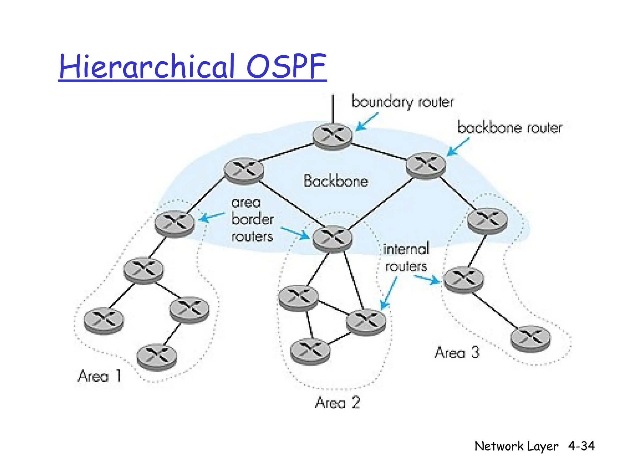
HierarchicalOSPF
Two-level hierarchy: local area, backbone.
Link-state advertisements only in area
each nodes has detailed area topology; only know
direction (shortest path) to nets in other areas.
Area border routers: “summarize” distances to nets
in own area, advertise to other Area Border routers.
Backbone routers: run OSPF routing limited to
backbone.
Boundary routers: connect to other AS’s.
36.
Network Layer 4-36
Internetinter-AS routing: BGP
BGP (Border Gateway Protocol): the de
facto standard
BGP provides each AS a means to:
1. Obtain subnet reachability information from
neighboring ASs.
2. Propagate the reachability information to all
routers internal to the AS.
3. Determine “good” routes to subnets based on
reachability information and policy.
Allows a subnet to advertise its existence
to rest of the Internet: “I am here”
37.
Network Layer 4-37
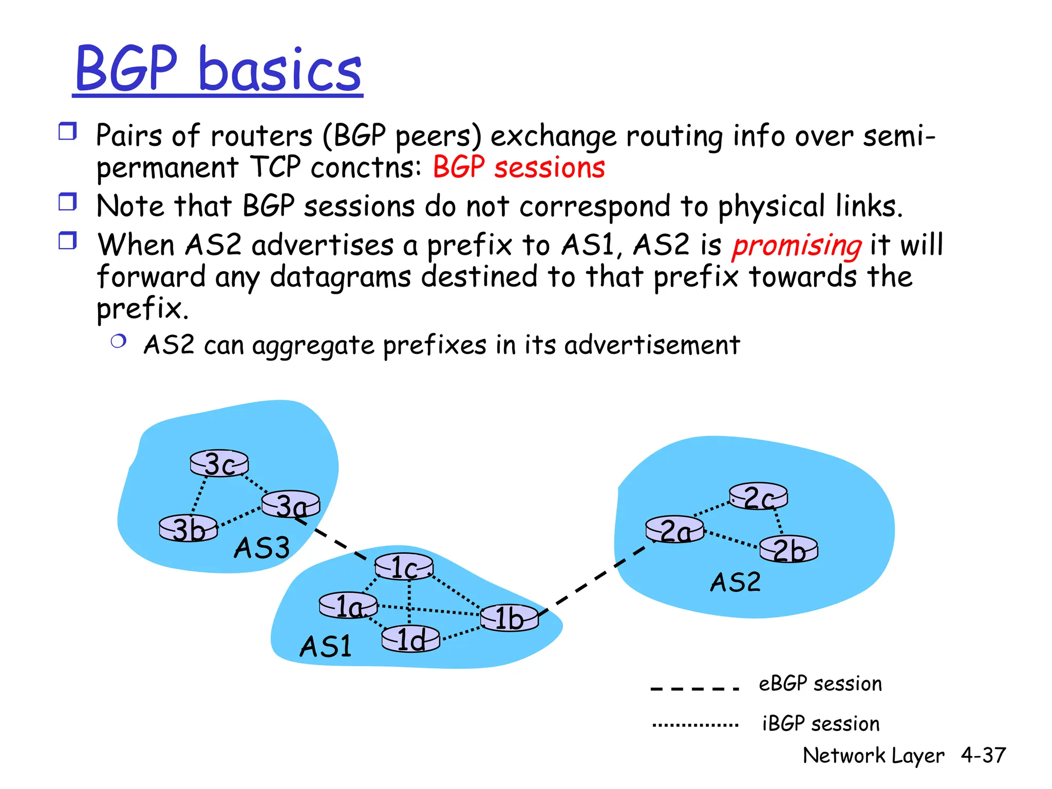
BGPbasics
Pairs of routers (BGP peers) exchange routing info over semi-
permanent TCP conctns: BGP sessions
Note that BGP sessions do not correspond to physical links.
When AS2 advertises a prefix to AS1, AS2 is promising it will
forward any datagrams destined to that prefix towards the
prefix.
AS2 can aggregate prefixes in its advertisement
3b
1d
3a
1c
2a
AS3
AS1
AS2
1a
2c
2b
1b
3c
eBGP session
iBGP session
38.
Network Layer 4-38
Distributingreachability info
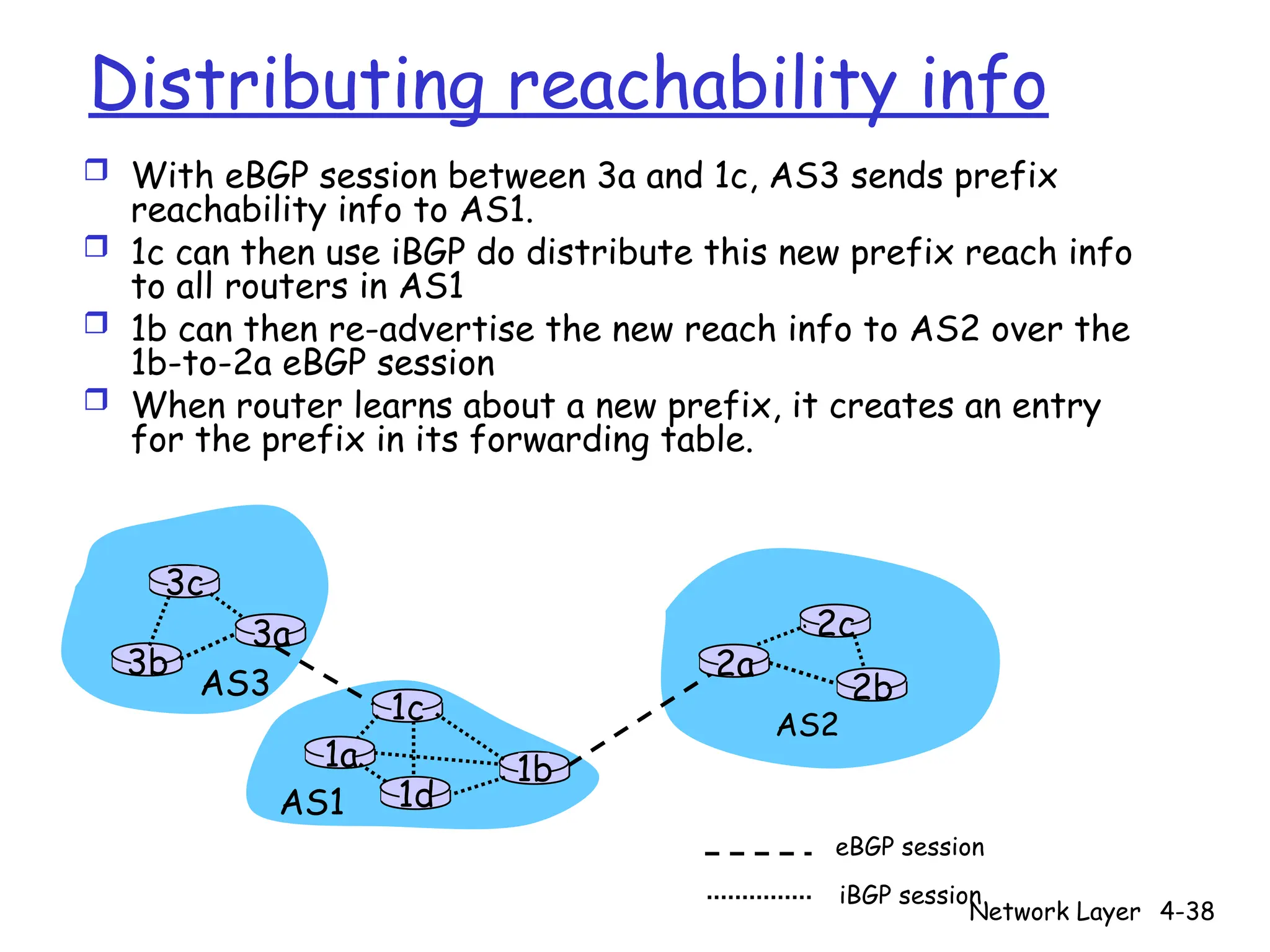
With eBGP session between 3a and 1c, AS3 sends prefix
reachability info to AS1.
1c can then use iBGP do distribute this new prefix reach info
to all routers in AS1
1b can then re-advertise the new reach info to AS2 over the
1b-to-2a eBGP session
When router learns about a new prefix, it creates an entry
for the prefix in its forwarding table.
3b
1d
3a
1c
2a
AS3
AS1
AS2
1a
2c
2b
1b
3c
eBGP session
iBGP session
39.
Network Layer 4-39
Pathattributes & BGP routes
When advertising a prefix, advert includes BGP
attributes.
prefix + attributes = “route”
Two important attributes:
AS-PATH: contains the ASs through which the advert
for the prefix passed: AS 67 AS 17
NEXT-HOP: Indicates the specific internal-AS router to
next-hop AS. (There may be multiple links from current
AS to next-hop-AS.)
When gateway router receives route advert, uses
import policy to accept/decline.
40.
Network Layer 4-40
BGProute selection
Router may learn about more than 1 route
to some prefix. Router must select route.
Elimination rules:
1. Local preference value attribute: policy
decision
2. Shortest AS-PATH
3. Closest NEXT-HOP router: hot potato routing
4. Additional criteria
41.
Network Layer 4-41
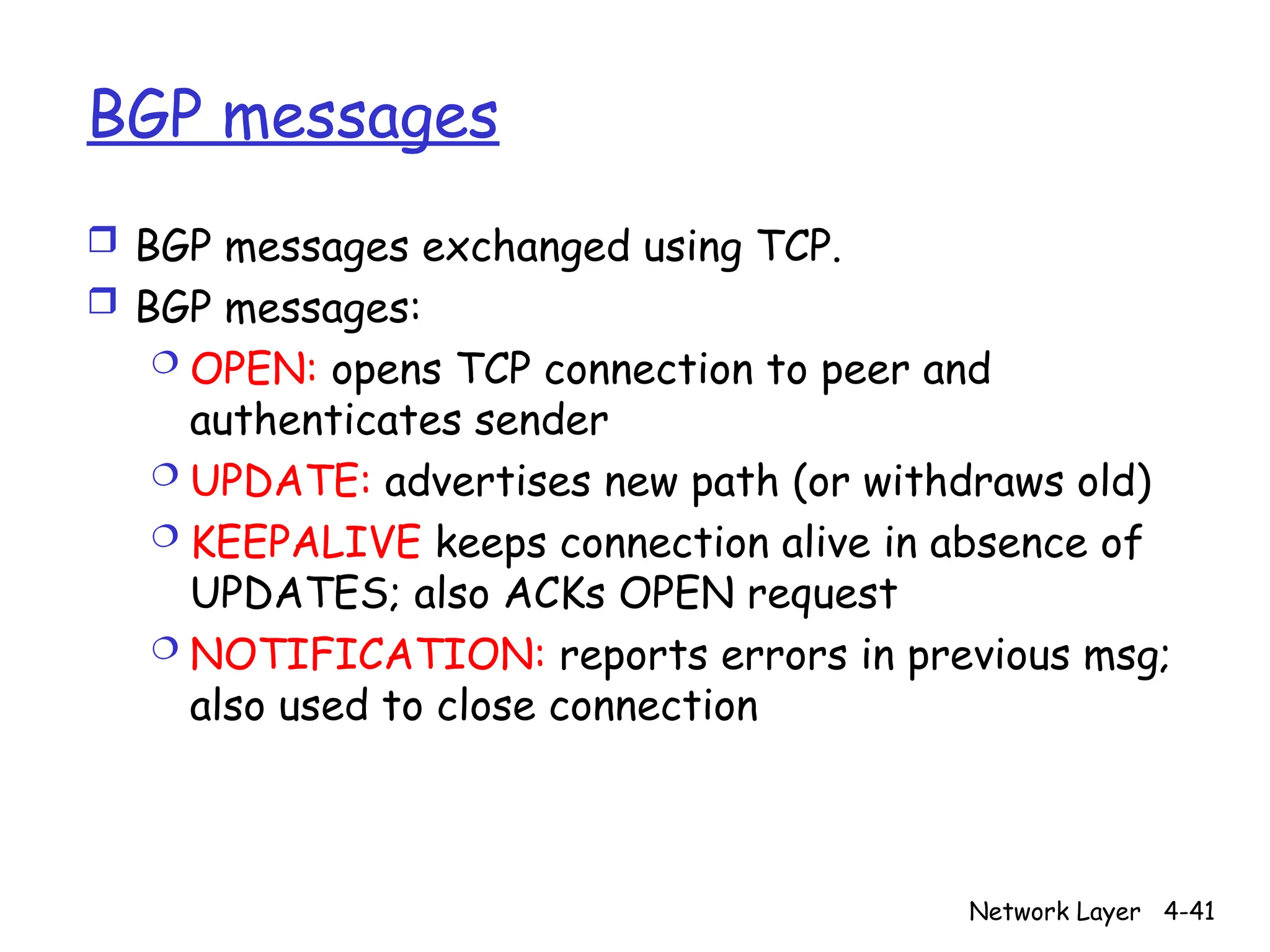
BGPmessages
BGP messages exchanged using TCP.
BGP messages:
OPEN: opens TCP connection to peer and
authenticates sender
UPDATE: advertises new path (or withdraws old)
KEEPALIVE keeps connection alive in absence of
UPDATES; also ACKs OPEN request
NOTIFICATION: reports errors in previous msg;
also used to close connection
42.
Network Layer 4-42
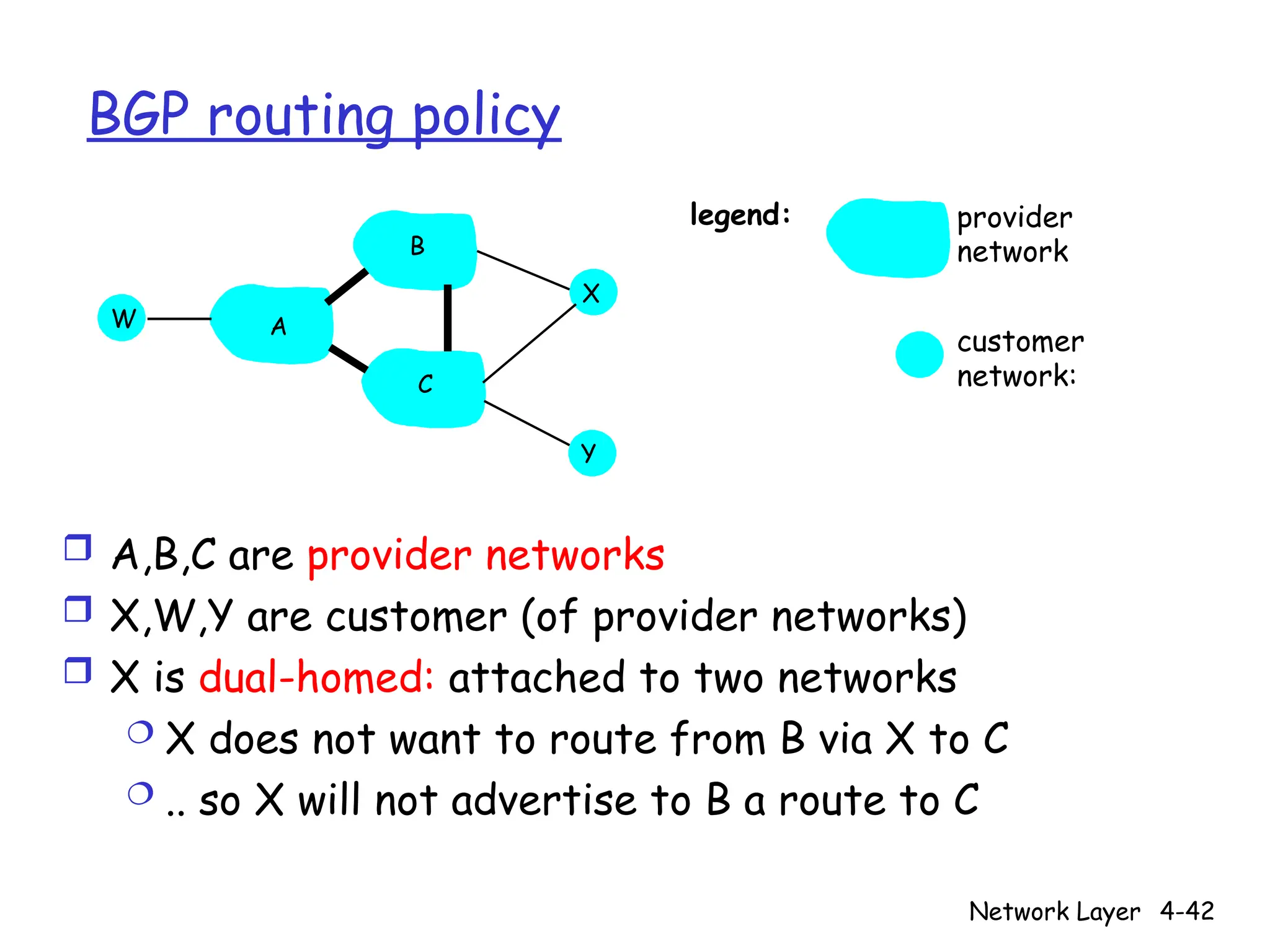
BGProuting policy
Figure 4.5
-BGPnew
: a simple BGP scenario
A
B
C
W
X
Y
legend:
customer
network:
provider
network
A,B,C are provider networks
X,W,Y are customer (of provider networks)
X is dual-homed: attached to two networks
X does not want to route from B via X to C
.. so X will not advertise to B a route to C
43.
Network Layer 4-43
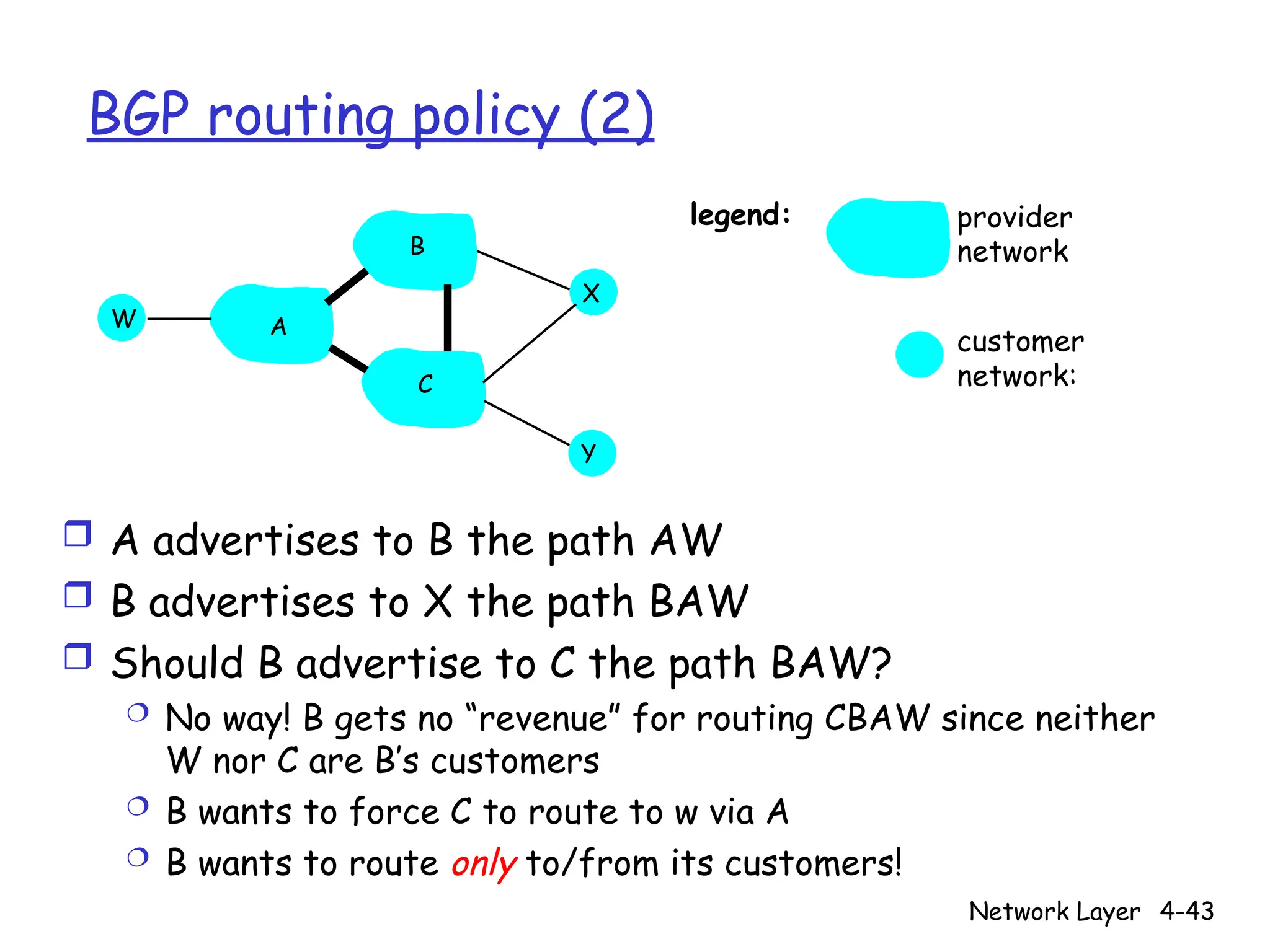
BGProuting policy (2)
Figure 4.5
-BGPnew
: a simple BGP scenario
A
B
C
W
X
Y
legend:
customer
network:
provider
network
A advertises to B the path AW
B advertises to X the path BAW
Should B advertise to C the path BAW?
No way! B gets no “revenue” for routing CBAW since neither
W nor C are B’s customers
B wants to force C to route to w via A
B wants to route only to/from its customers!
44.
Network Layer 4-44
Whydifferent Intra- and Inter-AS routing ?
Policy:
Inter-AS: admin wants control over how its traffic
routed, who routes through its net.
Intra-AS: single admin, so no policy decisions needed
Scale:
hierarchical routing saves table size, reduced update
traffic
Performance:
Intra-AS: can focus on performance
Inter-AS: policy may dominate over performance
![Network Layer 4-12
Distance Vector Algorithm (3)
Dx(y) = estimate of least cost from x to y
Distance vector: Dx = [Dx(y): y є N ]
Node x knows cost to each neighbor v:
c(x,v)
Node x maintains Dx = [Dx(y): y є N ]
Node x also maintains its neighbors’
distance vectors
For each neighbor v, x maintains
Dv = [Dv(y): y є N ]](https://image.slidesharecdn.com/routingalgorithms1-251002160317-b3ce637c/75/routing_algorithms-distance-vector-1-ppt-12-2048.jpg)