Deterministic vs Non-
Deterministic
Deterministic Algorithm:
• In deterministic algorithm, for a given particular input, the computer will
always produce the same output going through the same states.
• Can solve the problem in polynomial time.
• Can determine what is the next step.
Non-Deterministic Algorithm:
• In non-deterministic algorithm, for the same input, the compiler may
produce different output in different runs.
• Can’t solve the problem in polynomial time.
• Can’t determine what is the next step.
4
5.
Deterministic Algorithm
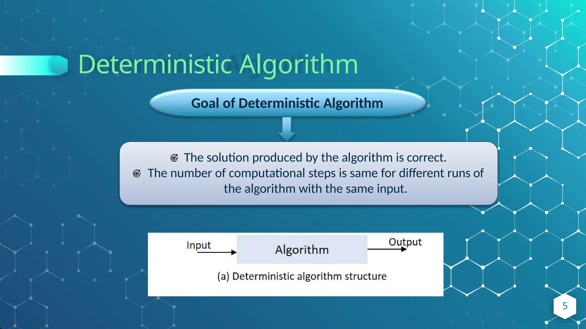
Goal ofDeterministic Algorithm
The solution produced by the algorithm is correct.
The number of computational steps is same for different runs of
the algorithm with the same input.
5
6.
Deterministic Algorithm
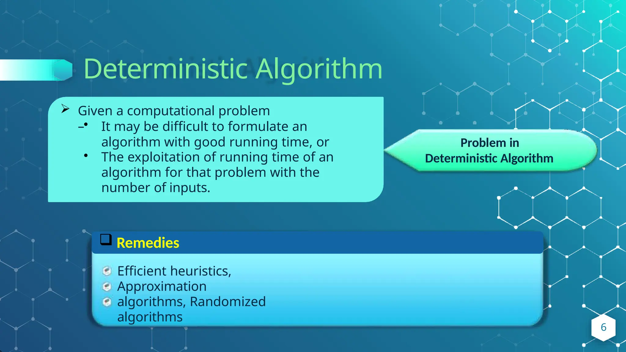
Problem in
DeterministicAlgorithm
Given a computational problem
–• It may be difficult to formulate an
algorithm with good running time, or
• The exploitation of running time of an
algorithm for that problem with the
number of inputs.
Remedies
Efficient heuristics,
Approximation
algorithms, Randomized
algorithms
6
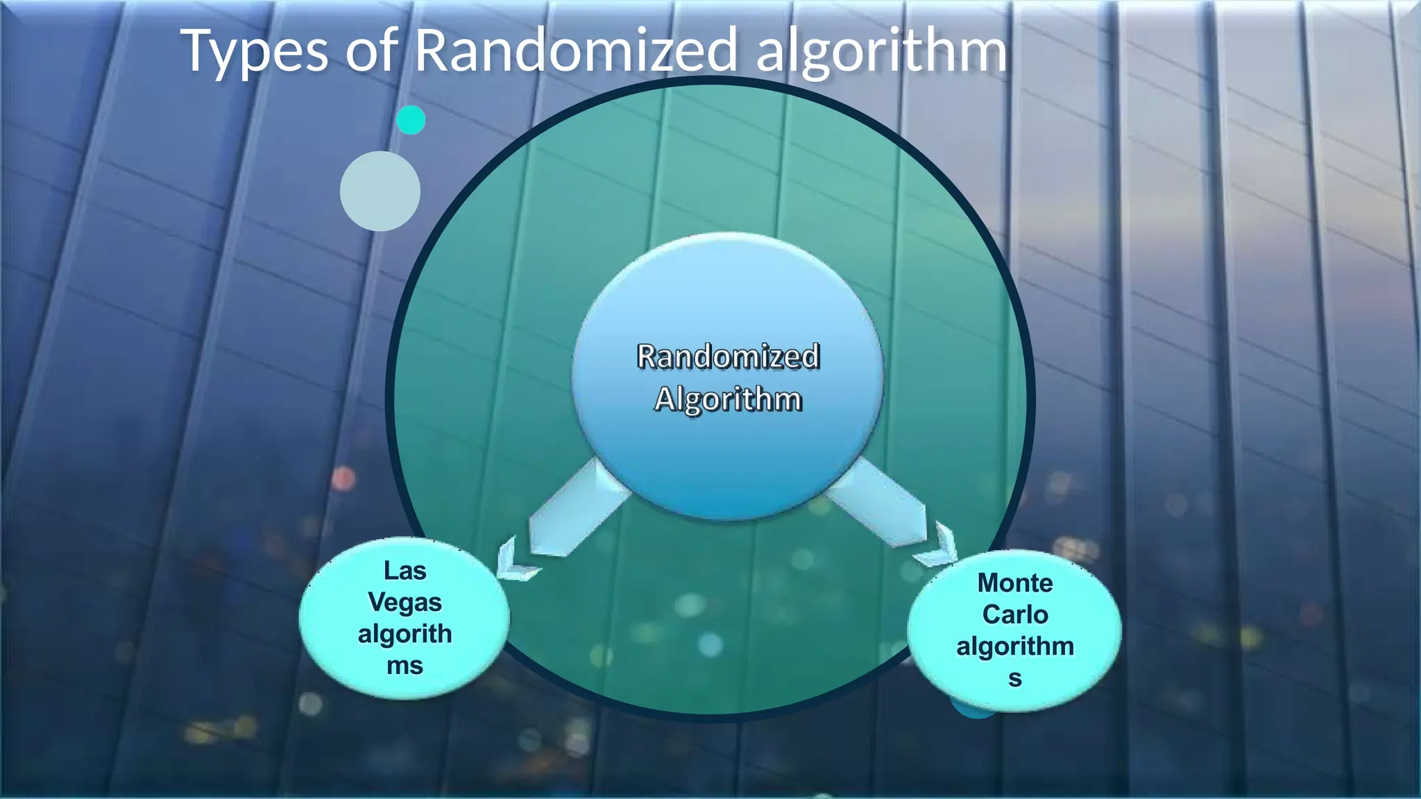
Randomized Algorithm
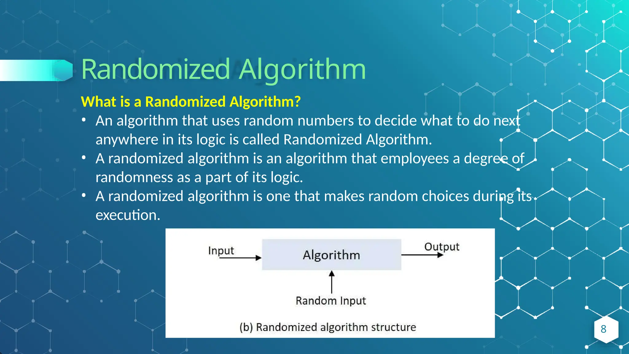
What isa Randomized Algorithm?
• An algorithm that uses random numbers to decide what to do next
anywhere in its logic is called Randomized Algorithm.
• A randomized algorithm is an algorithm that employees a degree of
randomness as a part of its logic.
• A randomized algorithm is one that makes random choices during its
execution.
8
9.
“
To overcomethe computation problem of exploitation of running time of a
deterministic algorithm, randomized algorithm is used.
Randomized algorithm uses uniform random bits also called as pseudo random
number as an input to guides its behavior (Output).
Randomized algorithms rely on the statistical properties of random numbers
(e.g. randomized algorithm is quick sort).
It tries to achieve good performance in the average case.
9
10.
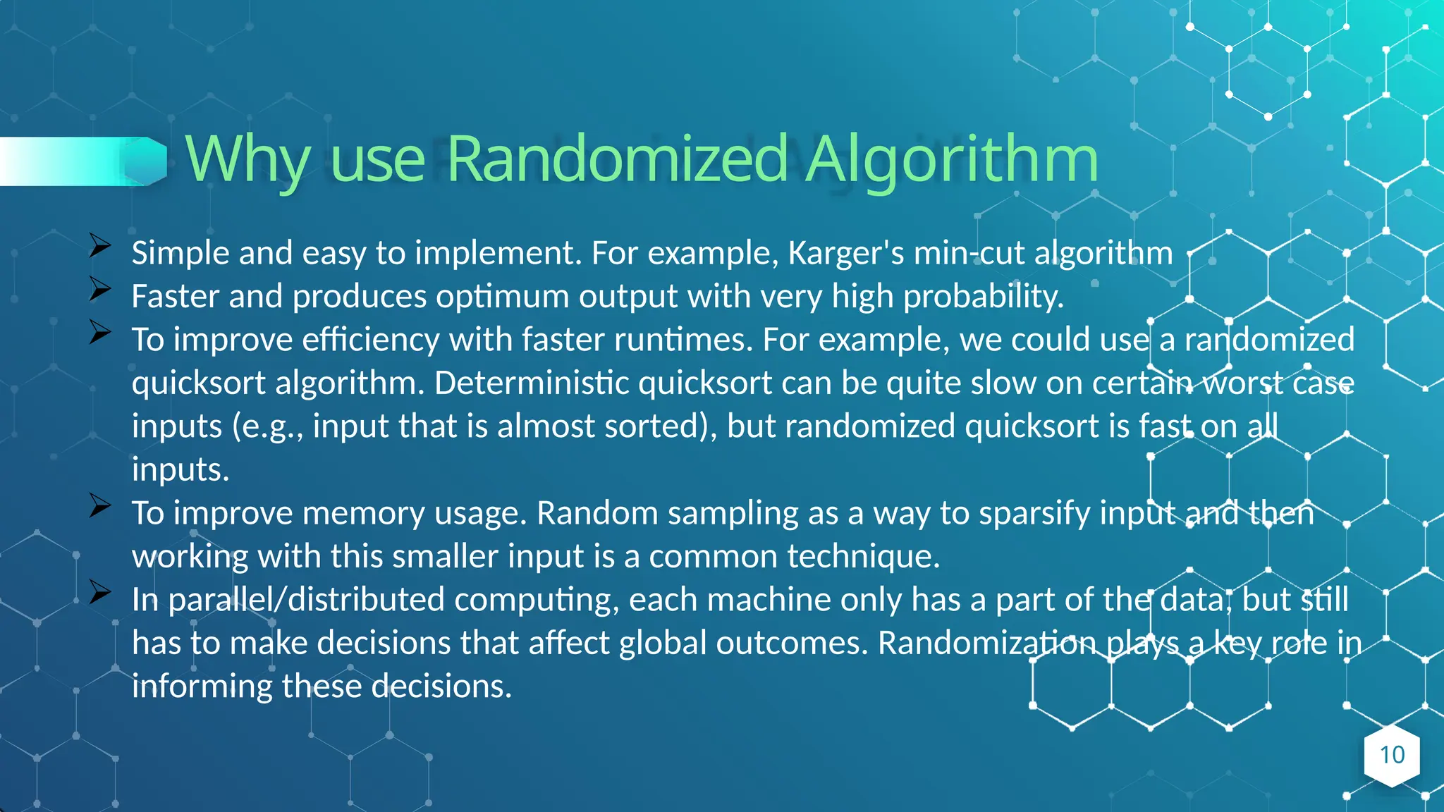
Why use RandomizedAlgorithm
10
Simple and easy to implement. For example, Karger's min-cut algorithm
Faster and produces optimum output with very high probability.
To improve efficiency with faster runtimes. For example, we could use a randomized
quicksort algorithm. Deterministic quicksort can be quite slow on certain worst case
inputs (e.g., input that is almost sorted), but randomized quicksort is fast on all
inputs.
To improve memory usage. Random sampling as a way to sparsify input and then
working with this smaller input is a common technique.
In parallel/distributed computing, each machine only has a part of the data, but still
has to make decisions that affect global outcomes. Randomization plays a key role in
informing these decisions.
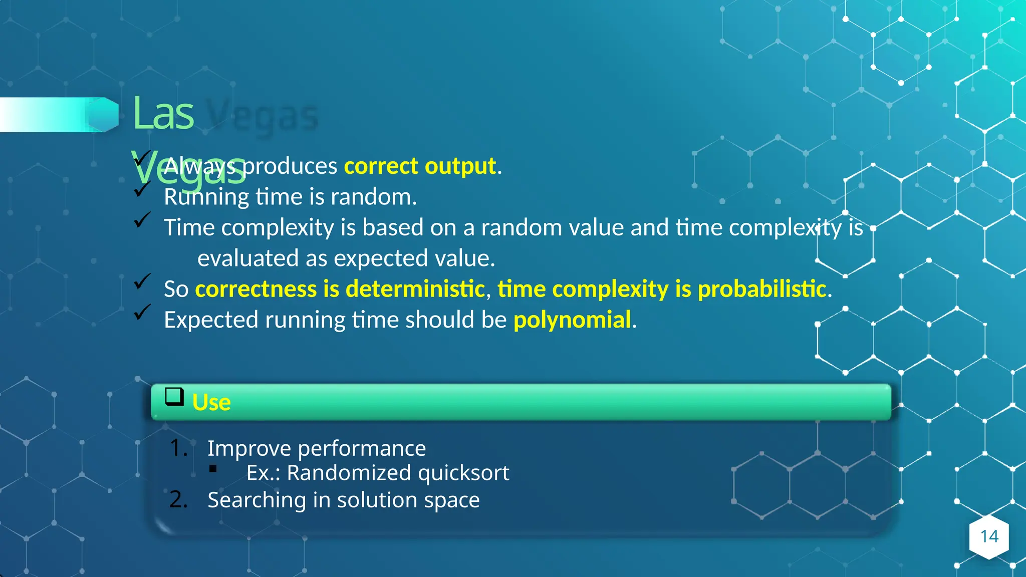
Las
Vegas
Always producescorrect output.
Running time is random.
Time complexity is based on a random value and time complexity is
evaluated as expected value.
So correctness is deterministic, time complexity is probabilistic.
Expected running time should be polynomial.
Use
1. Improve performance
Ex.: Randomized quicksort
2. Searching in solution space
14
Divide and Conquer
Thedesign of Quicksort is based on the divide-and-conquer paradigm.
Divide: Partition the array A[p..r] into two subarrays A[p..q-1] and A[q+1,r]
such that,
A[x] <= A[q] for all x in [p..q-1]
A[x] > A[q] for all x in [q+1,r]
≤ 𝒙 𝒙 ≥ 𝒙
Conquer: Recursively sort A[p..q-1] and A[q+1,r]
Combine: nothing to do here
15
16.
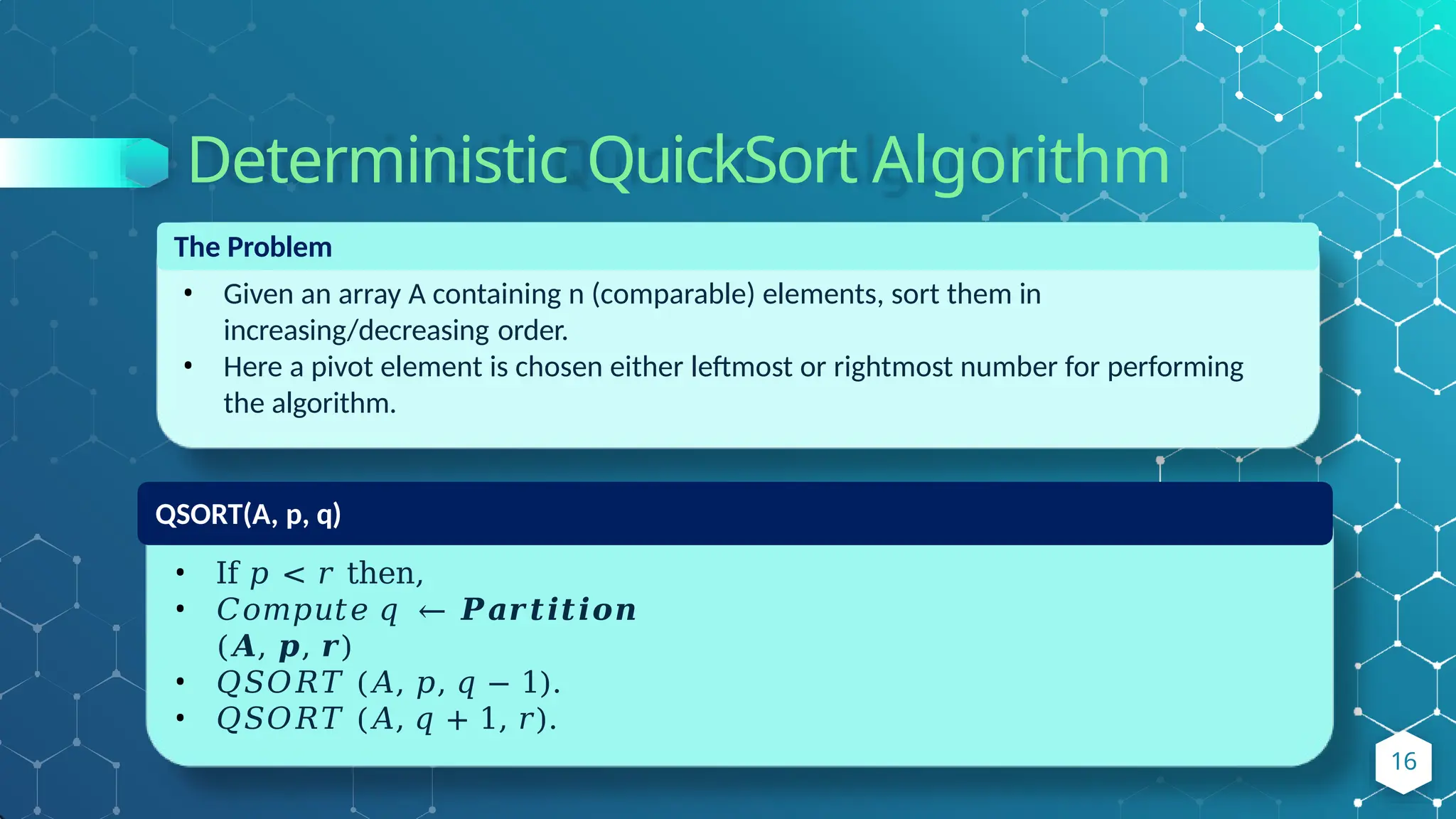
Deterministic QuickSort Algorithm
TheProblem
• Given an array A containing n (comparable) elements, sort them in
increasing/decreasing order.
• Here a pivot element is chosen either leftmost or rightmost number for performing
the algorithm.
QSORT(A, p, q)
• If 𝑝 < 𝑟 then,
• 𝐶𝑜𝑚𝑝𝑢𝑡𝑒 𝑞 ← 𝑷𝒂𝒓𝒕𝒊𝒕𝒊𝒐𝒏
(𝑨, 𝒑, 𝒓)
• 𝑄𝑆𝑂𝑅𝑇 (𝐴, 𝑝, 𝑞 − 1).
• 𝑄𝑆𝑂𝑅𝑇 (𝐴, 𝑞 + 1, 𝑟).
16
Deterministic QuickSort Algorithm
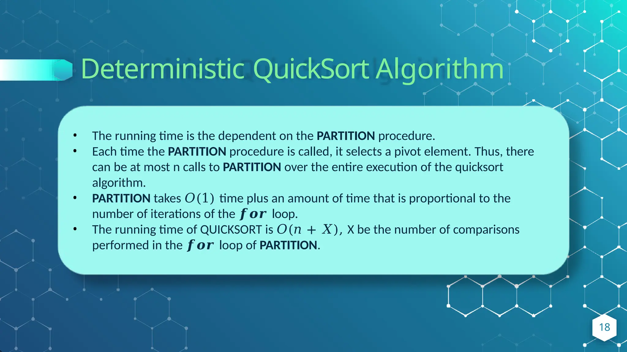
•The running time is the dependent on the PARTITION procedure.
• Each time the PARTITION procedure is called, it selects a pivot element. Thus, there
can be at most n calls to PARTITION over the entire execution of the quicksort
algorithm.
• PARTITION takes 𝑂(1) time plus an amount of time that is proportional to the
number of iterations of the 𝒇𝒐𝒓 loop.
• The running time of QUICKSORT is 𝑂(𝑛 + 𝑋), X be the number of comparisons
performed in the 𝒇𝒐𝒓 loop of PARTITION.
18
Randomized QuickSort Algorithm
21
Randomized-Quicksort(A,p, r)
if p < r then
q := Randomized-Partition(A, p, r);
Randomized-Quicksort(A, p,q-1);
Randomized-Quicksort(A,p+1,r);
Randomized-Partition(A, p, r)
i := Random(p, r);
swap(A[i], A[r]);
p := Partition(A, p, r);
Return p;
Almost the same as Partition as Deterministic QuickSort, but now the pivot
element is not the rightmost/leftmost element, but rather an element from
A[p..r] that is chosen uniformly at random.
21.
Randomized QuickSort Algorithm
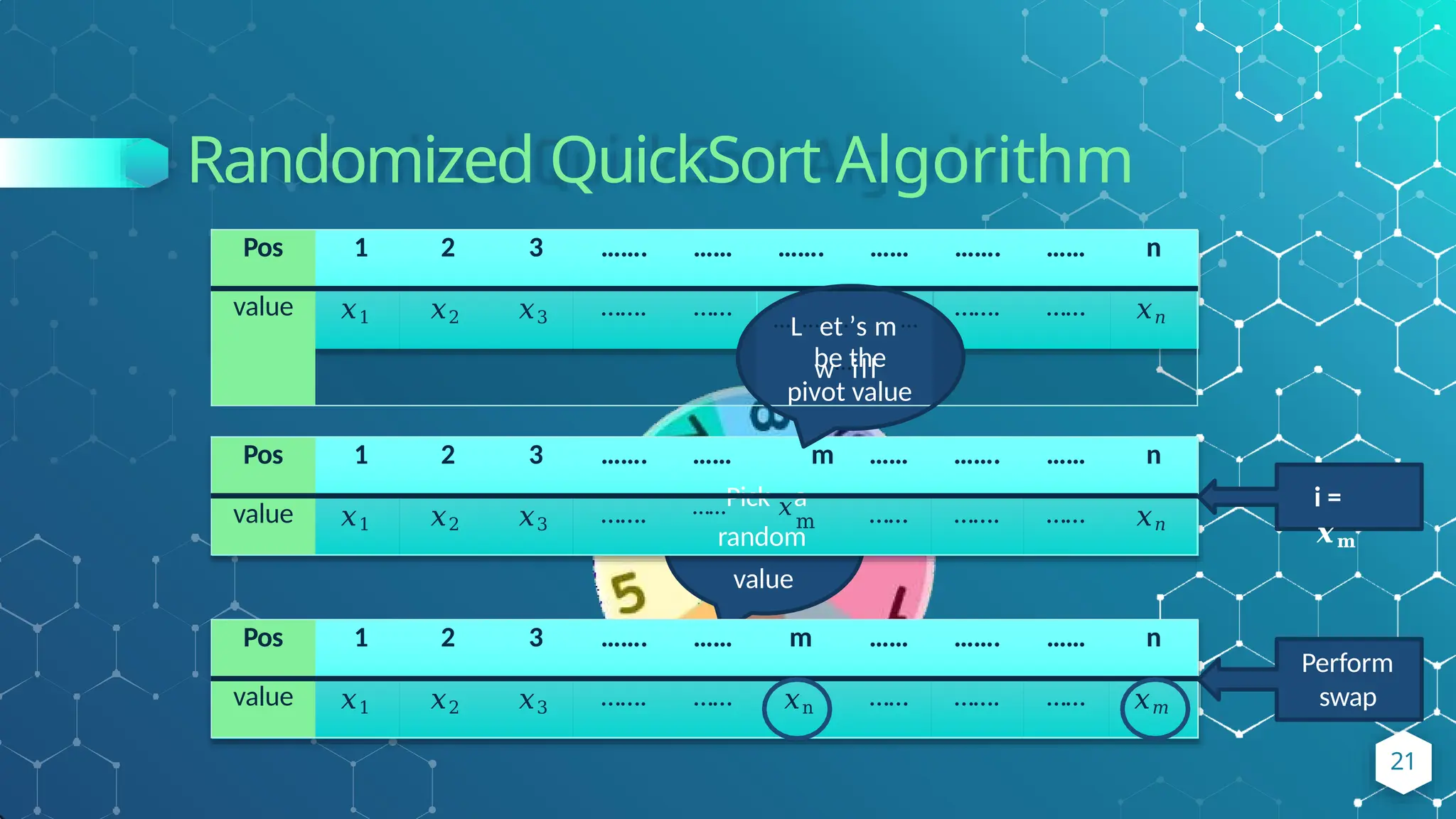
value
Pos1 2 3 ……. …… m …… ……. …… n
value 𝑥1 𝑥2 𝑥3 ……. ……Pick 𝑥a
m
random
…… ……. …… 𝑥𝑛
Pos 1 2 3 ……. …… ……. …… ……. …… n
value 𝑥1 𝑥2 𝑥3 ……. …… …L…et.’s m…
w…ill
……. …… 𝑥𝑛
be the
pivot value
Pos 1 2 3 ……. …… m …… ……. …… n
value 𝑥1 𝑥2 𝑥3 ……. …… 𝑥n …… ……. …… 𝑥𝑚
i =
𝒙𝐦
Perform
swap
21
22.
Randomized QuickSort Algorithm
Goal
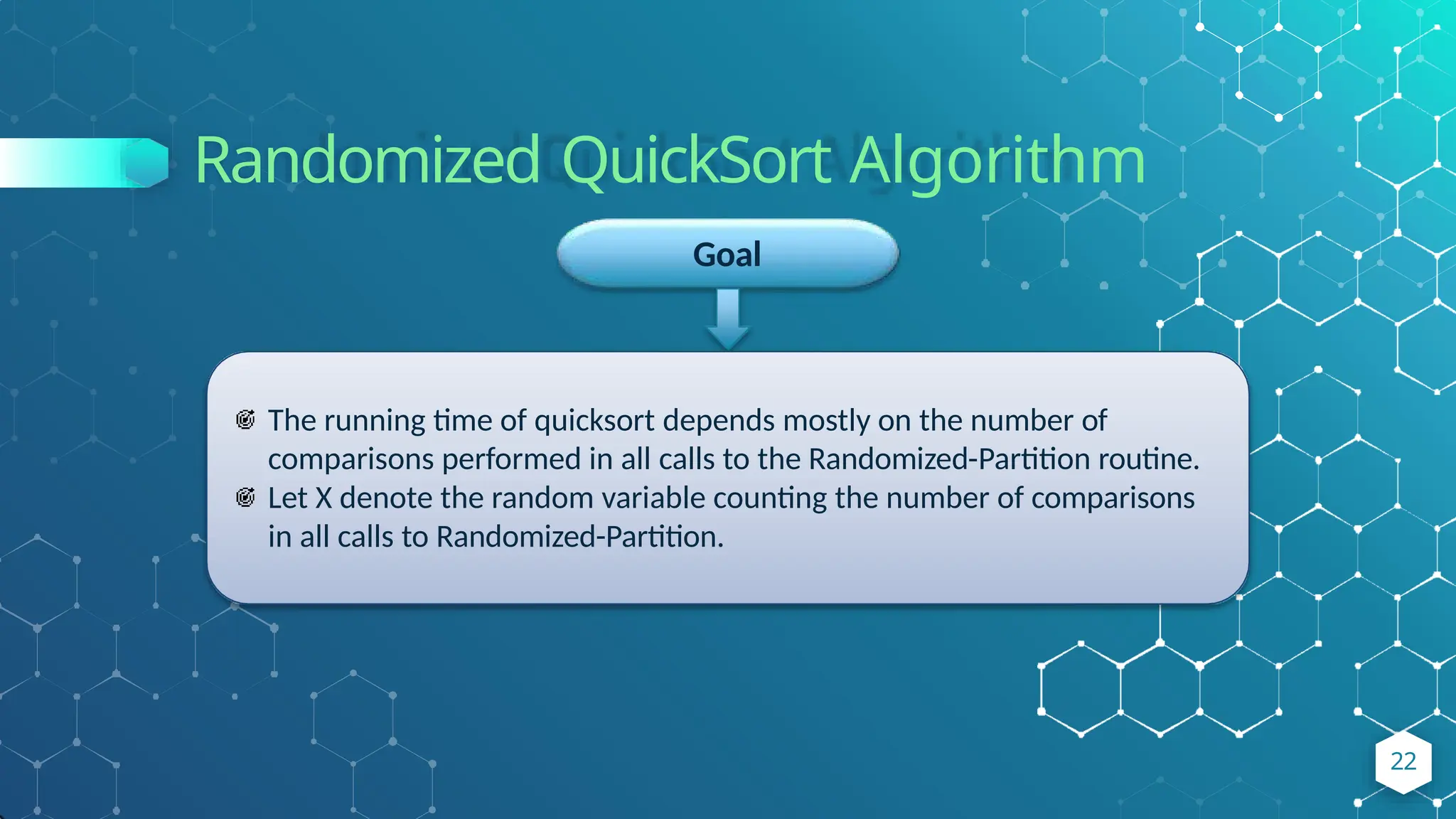
Therunning time of quicksort depends mostly on the number of
comparisons performed in all calls to the Randomized-Partition routine.
Let X denote the random variable counting the number of comparisons
in all calls to Randomized-Partition.
22
23.
24
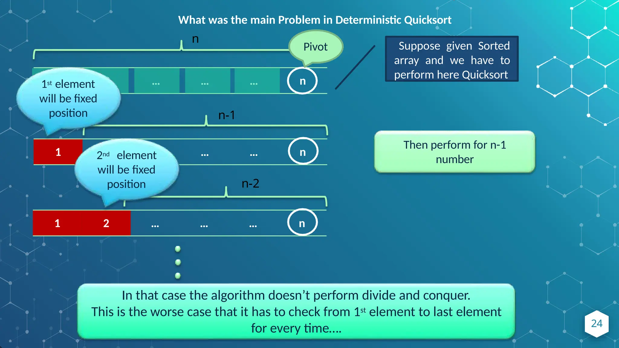
What was themain Problem in Deterministic Quicksort
1 2 … … … n
Suppose given Sorted
array and we have to
perform here Quicksort
n
Pivot
1 2 … … … n
n-1
1 2 … … … n
n-2
1st element
will be fixed
position
Then perform for n-1
number
2nd element
will be fixed
position
In that case the algorithm doesn’t perform divide and conquer.
This is the worse case that it has to check from 1st element to last element
for every time….
24.
What will behappened in case of Randomized Quicksort
4
Pick a random
number
1 2
3
6 5 4
1 2 3 4 5 6
p i r
Swap(A[i],A[r])
and then perform
Partition function
Pivot
p
24
r
25.
What will behappened in case of Randomized Quicksort
1 2 3 6 5 4
i=p-1 j x
1 2 3 6 5 4
i j x
1 2 3 6 5 4
i j x
1 2 3 6 5 4
i j
A[j] <= x
?
No
6 4
i j A[j] <= x
?
No
1 2 3 4 5 6
1 2 3 6 5 4
25
26.
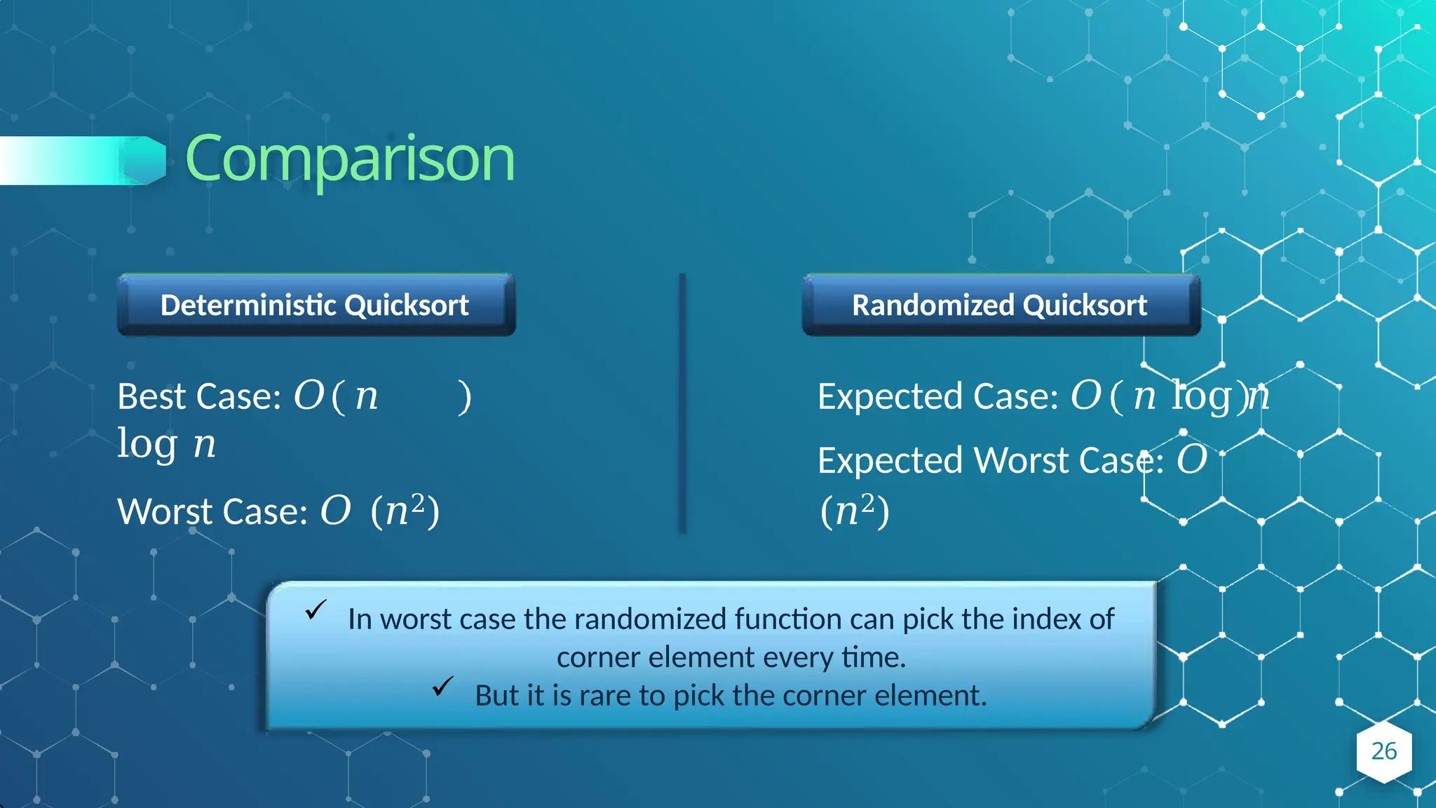
Comparison
Randomized Quicksort
Expected Case:𝑂 𝑛 log 𝑛
Expected Worst Case: 𝑂
(𝑛2)
Deterministic Quicksort
Best Case: 𝑂 𝑛
log 𝑛
Worst Case: 𝑂 (𝑛2)
In worst case the randomized function can pick the index of
corner element every time.
But it is rare to pick the corner element.
26
27.
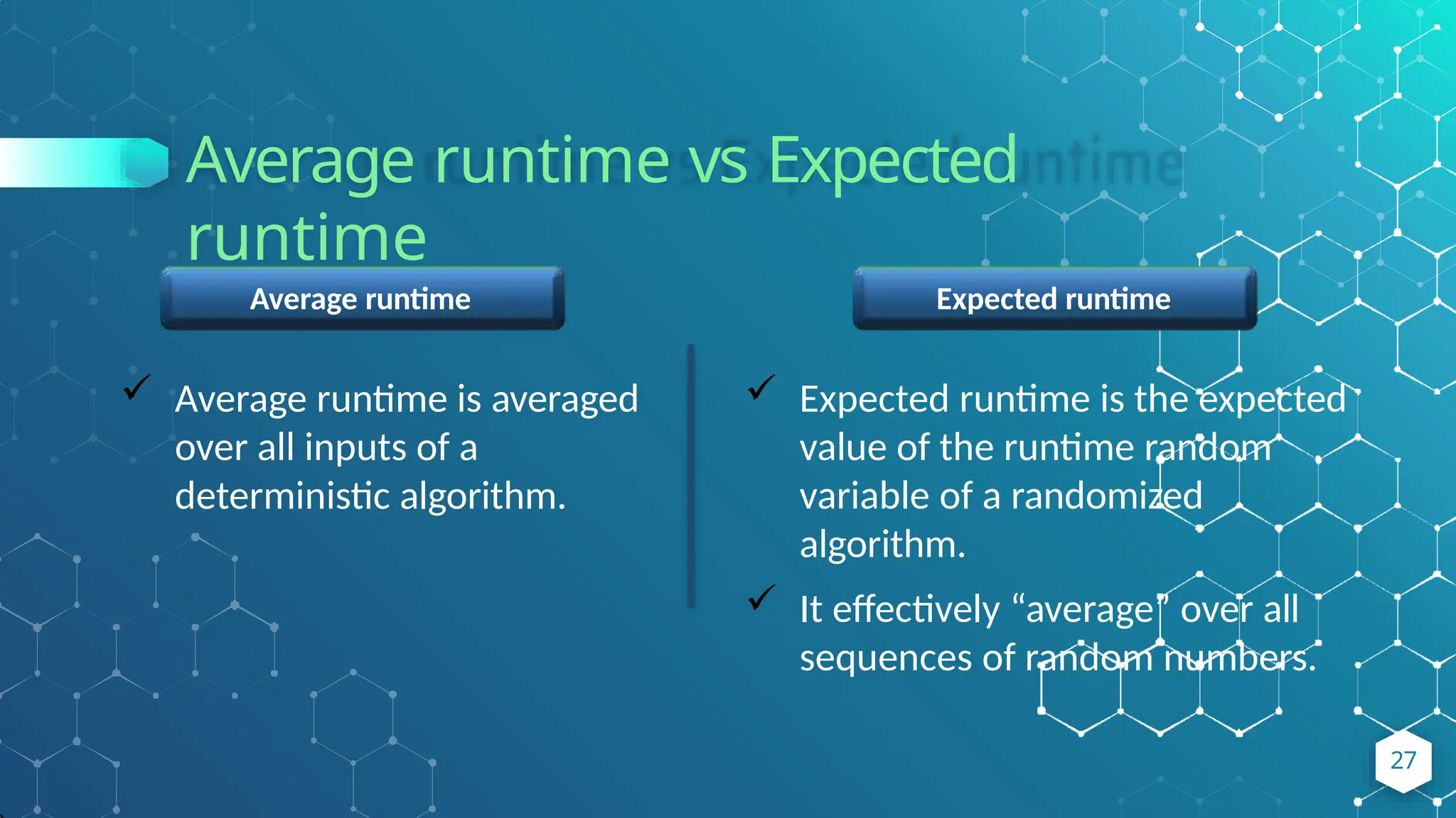
Average runtime vsExpected
runtime
Expected runtime
Expected runtime is the expected
value of the runtime random
variable of a randomized
algorithm.
It effectively “average” over all
sequences of random numbers.
Average runtime
Average runtime is averaged
over all inputs of a
deterministic algorithm.
27
“
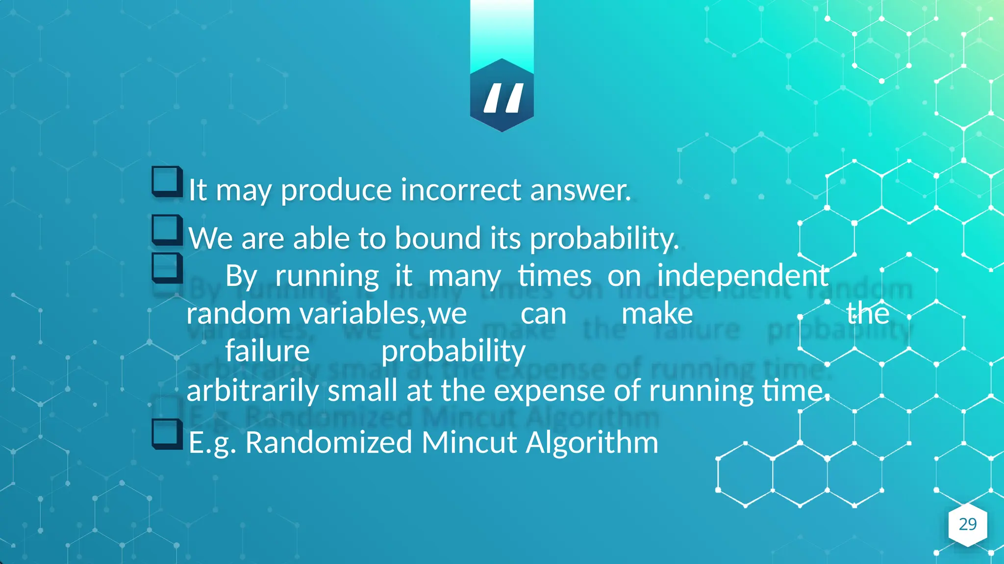
It may produceincorrect answer.
We are able to bound its probability.
By running it many times on independent
random variables,we can make the
failure probability
arbitrarily small at the expense of running time.
E.g. Randomized Mincut Algorithm
29
30.
Monte Carlo Example
◆Suppose we want to find a number among n given numbers
which is larger than or equal to the median.
◆ Suppose A1 < … < An .
◆ We want Ai , such that i ≥ n/2. It’s obvious that the best
deterministic algorithm needs O(n) time to produce
the answer. n may be very large! Suppose n is
100,000,000,000!
◆ Choose 100 of the numbers with equal probability.
◆ Find the maximum among these numbers. Return the
maximum.
30
31.
Monte Carlo Example
31
The running time of the given algorithm is O(1).
The probability of Failure is 1/(2100).
Consider that the algorithm may return a wrong answer but
the probability is very smaller than the hardware failure or
even an earthquake!
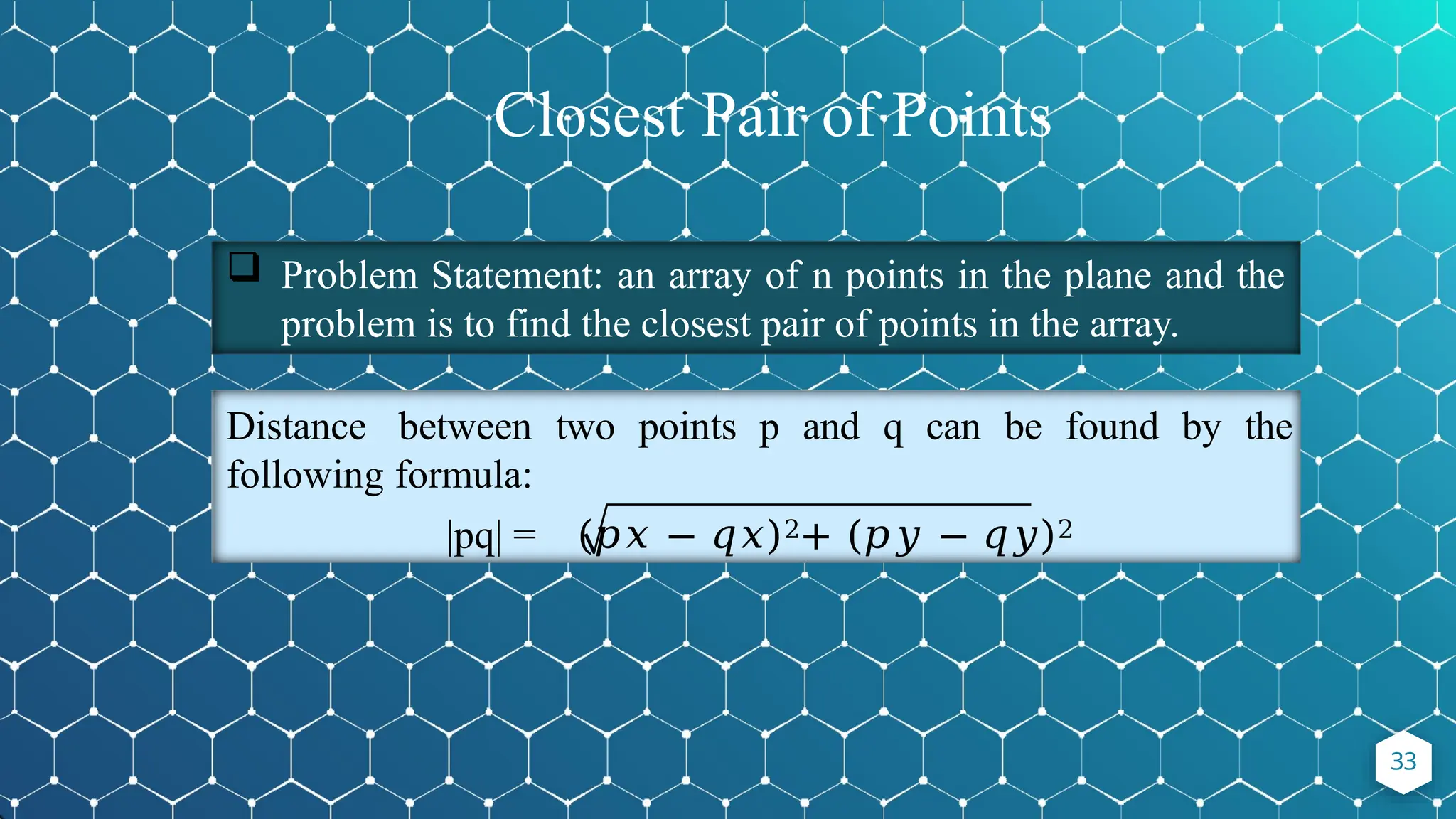
Problem Statement:an array of n points in the plane and the
problem is to find the closest pair of points in the array.
Distance between two points p and q can be found by the
following formula:
|pq| = (𝑝𝑥 − 𝑞𝑥)2+ (𝑝𝑦 − 𝑞𝑦)2
33
Closest Pair of Points
34.
Algorith
m
◆ Input: Anarray of n points P[ ].
◆ Output: Smallest distance between two points in the
given array.
P[ ] = {0,1, 2, 3, 4, 5, 6, 7, 8, 9, 10, 11, 12, 13, 14, 15, 16,
17}
34
35.
Algorithm Cont….
40
Sort thearray according to the x-coordinates at first as preprocessing
step.
P[ ] = {13, 12, 11, 0, 14, 16, 1, 10, 17, 9, 2, 15, 3, 8, 4, 5, 7, 6}
1. Find the middle point in sorted array. We can take P[n/2] as the
middle point.
P[ ] = {13, 12, 11, 0, 14, 16, 1, 10, 17, 9, 2, 15, 3, 8, 4, 5, 7, 6}
2.Divide the array in two halves. The first subarray contains
points for P[0] to P[n/2] and the second subarray contains
points from P[n/2+1] to P[n-1].
𝑃𝐿 = {13, 12, 11, 0, 14, 16, 1, 10, 17} 𝑃𝑅 = {9, 2, 15, 3, 8, 4, 5, 7,
6}
36.
Algorithm Cont….
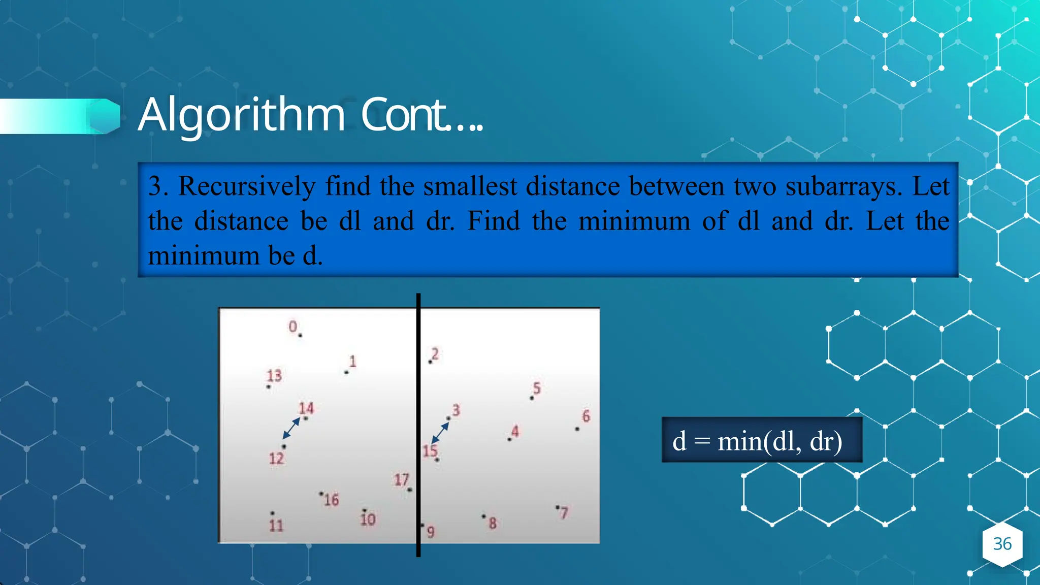
3. Recursivelyfind the smallest distance between two subarrays. Let
the distance be dl and dr. Find the minimum of dl and dr. Let the
minimum be d.
d = min(dl, dr)
36
37.
Our knowledge:Insertion time depends on
whether the closest pair is changed or not.
If output is the same: 1 clock tick. If output is
not the same: |D| clock ticks.
With random insertion order, show that the
expected total number of clock ticks used by D
is O(n)
37
Minimum Cut
◆ Min-Cutof a weighted graph is defined as the minimum sum
of weights of (at least one)edges that when removed from
the graph divides the graph into two groups.
◆ The algorithm works on a method of shrinking the graph
until only one node is left in the graph.
◆ Minimum value in the list would be the minimum cut value
of the graph.
44
40.
Minimum Cut Cont....
45
•Select the edge with minimum weight and according this minimum
weight edge next move is done in e network graph.
Some points are taken in consideration when working with Min-Cut:
• A cut of connected graph is obstained bye dividing vertex set V of
graph G into 2 sets 𝑉1 & 𝑉2.
• There are no common vertices in 𝑉1 & 𝑉2, that is, two
sets are disjoint.
• 𝑉1 U 𝑉2 = V
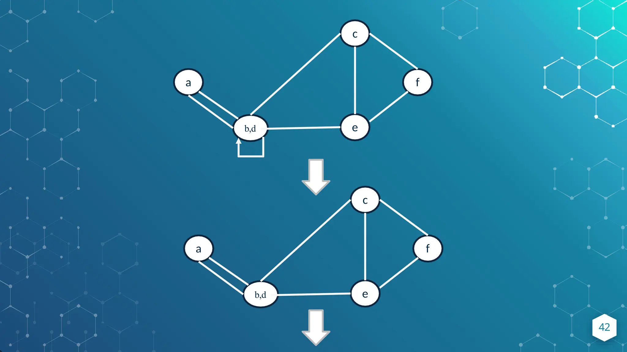
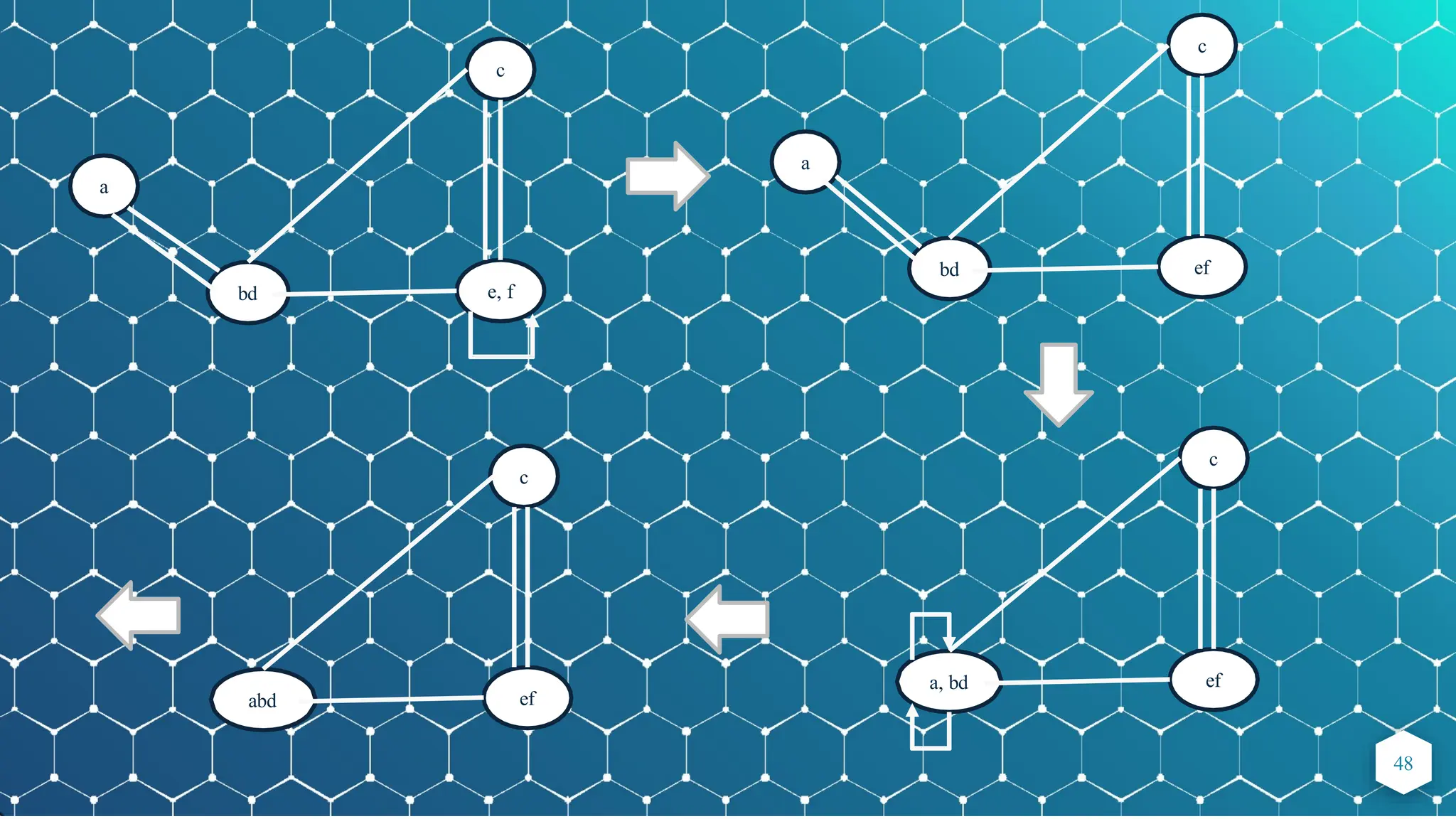
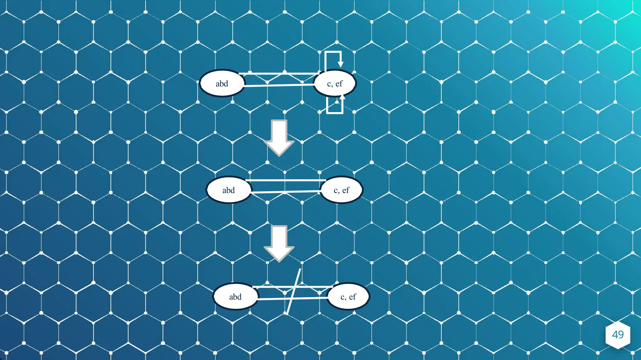
41.
Minimum Cut Cont….
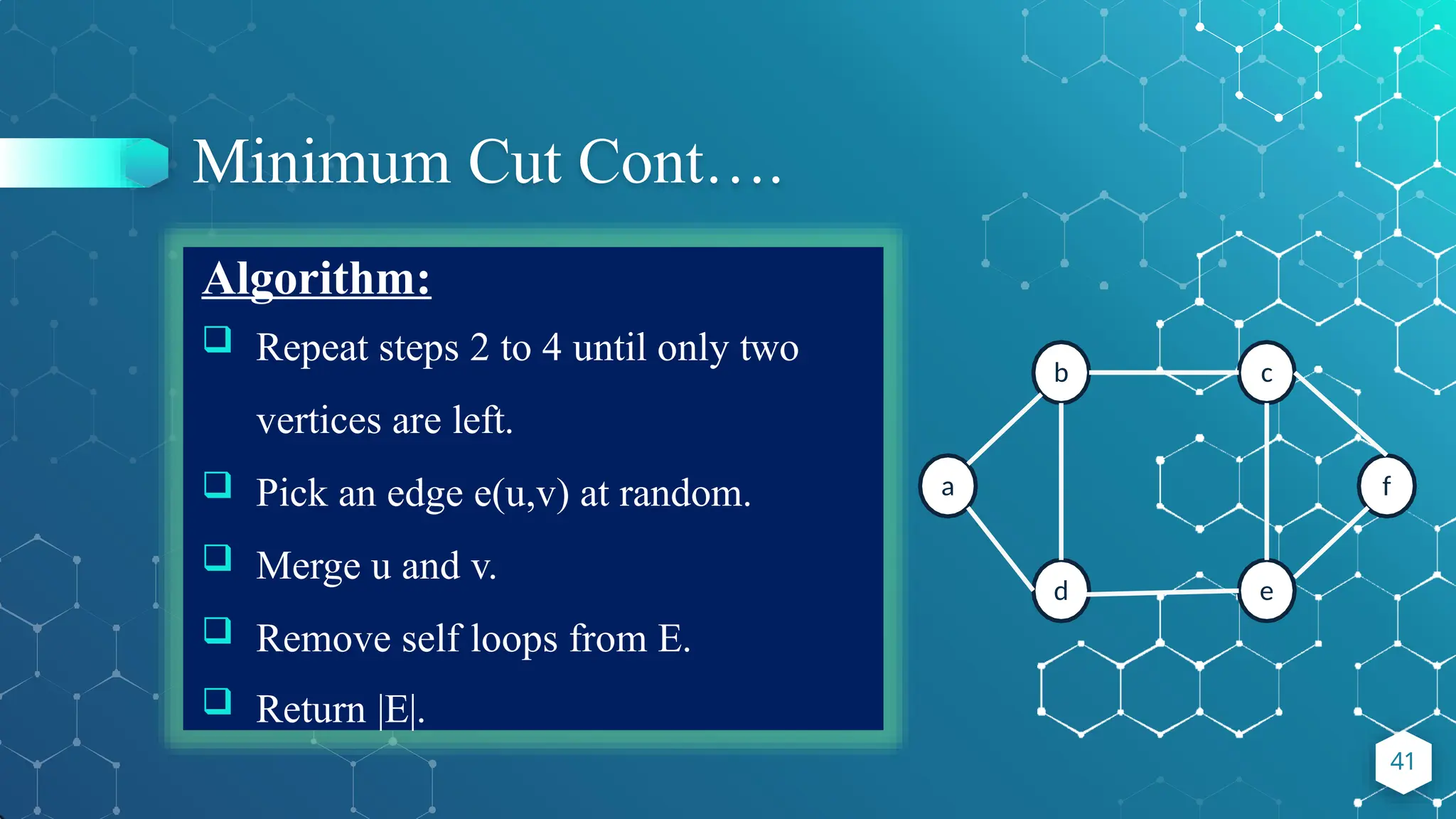
Algorithm:
Repeat steps 2 to 4 until only two
vertices are left.
Pick an edge e(u,v) at random.
Merge u and v.
Remove self loops from E.
Return |E|.
a
b
d
c
e
f
41
Minimum Cut
50
Problemdefinition: Given a connected graph G=(V,E) on n
vertices and m edges, compute the smallest set of edges
that will make G disconnected.
Best deterministic algorithm : [Stoer and Wagner, 1997]
• O(mn) time complexity.
Randomized Monte Carlo algorithm: [Karger, 1993]
• O(m log n) time complexity.
Error probability: n−𝑐 for any 𝑐 that we
desire.
46.
Applications of MinimumCut
Algorithm
46
Partitioning items in a database,
Identify clusters of related documents,
Network reliability,
Network design,
Circuit design, etc.
47.
Classifying Randomized Algorithmsby Their Methods
47
Avoiding Worst-Case Inputs: Obtained by hiding the details of the
algorithm from the adversary. Since the algorithm is chosen
randomly, he can’t pick an input that is bad for all of them.
Sampling: Randomness is used for choosing a simple random
sample, without replacement, of k items from a population of
unknown size n in a single pass over the items. In this way, the
adversary can’t direct us to non-representative samples.
48.
Classifying Randomized Algorithmsby Their Methods
48
Hashing: Obtained by selecting a hash function at random from a
family of hash functions. This guarantees a low number of
collisions in expectation, even if the data is chosen by an
adversary.
Building Random Structures: By creating a randomized algorithm to
create structures, the probability can be reached to substantial.
Symmetry Breaking: Randomization can break the deadlocks of
making the progress of multiple processes stymied.
49.
Advantages of Randomized
Algorithms
49
The algorithm is usually simple and easy to
implement,
The algorithm is fast with very high probability, and
It produces optimum output with very high probability.
50.
Difficulties in Randomized
Algorithm
73
There is a finite probability of getting incorrect answer.
However, the probability of getting a wrong answer can be made
arbitrarily small by the repeated employment of randomness.
Analysis of running time or probability of getting a
correct
answer is usually difficult.
Getting truly random numbers is impossible. One needs to
depend on pseudo random numbers. So, the result
highly
depends on the quality of the random numbers.
Its quality depends on quality of random number generator used
as part of the algorithm.
The other disadvantage of randomized algorithm is hardware
failure.
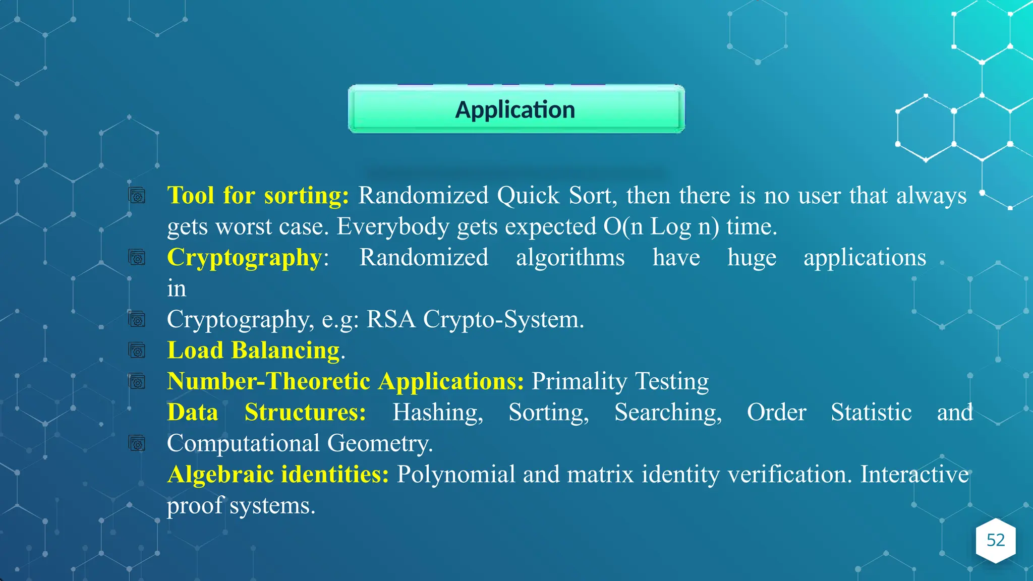
Tool for sorting:Randomized Quick Sort, then there is no user that always
gets worst case. Everybody gets expected O(n Log n) time.
Cryptography: Randomized algorithms have huge applications
in
Cryptography, e.g: RSA Crypto-System.
Load Balancing.
Number-Theoretic Applications: Primality Testing
Data Structures: Hashing, Sorting, Searching, Order Statistic and
Computational Geometry.
Algebraic identities: Polynomial and matrix identity verification. Interactive
proof systems.
Application
52
53.
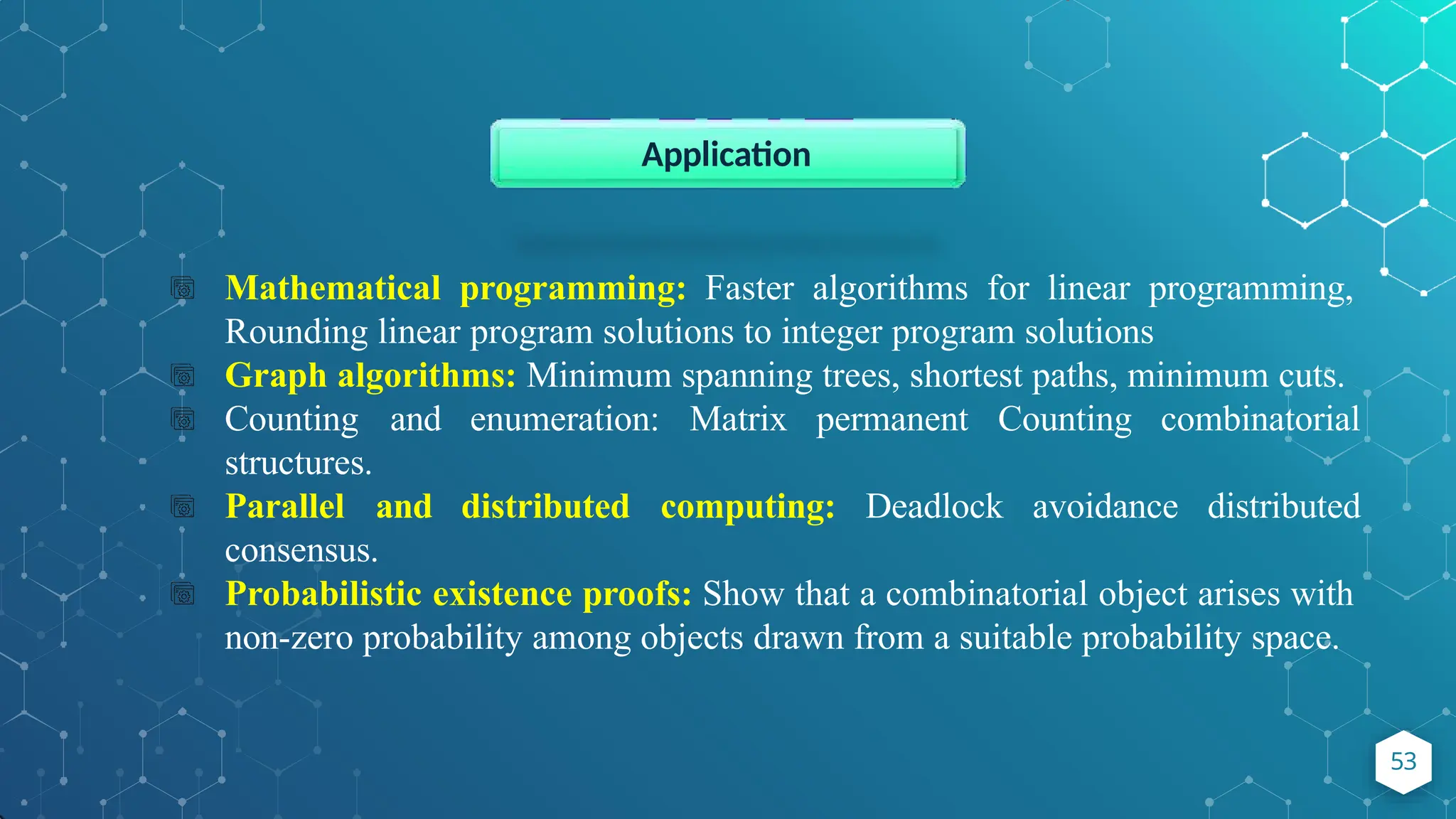
Mathematical programming: Fasteralgorithms for linear programming,
Rounding linear program solutions to integer program solutions
Graph algorithms: Minimum spanning trees, shortest paths, minimum cuts.
Counting and enumeration: Matrix permanent Counting combinatorial
structures.
Parallel and distributed computing: Deadlock avoidance distributed
consensus.
Probabilistic existence proofs: Show that a combinatorial object arises with
non-zero probability among objects drawn from a suitable probability space.
Application
53


![Divide and Conquer
The design of Quicksort is based on the divide-and-conquer paradigm.
Divide: Partition the array A[p..r] into two subarrays A[p..q-1] and A[q+1,r]
such that,
A[x] <= A[q] for all x in [p..q-1]
A[x] > A[q] for all x in [q+1,r]
≤ 𝒙 𝒙 ≥ 𝒙
Conquer: Recursively sort A[p..q-1] and A[q+1,r]
Combine: nothing to do here
15](https://image.slidesharecdn.com/randomizedalgorithm-211022054611-251128142647-7fd12c6b/75/randomizedalgorithm-and-understand-quick-sort-pptx-15-2048.jpg)
![Deterministic QuickSort Algorithm
17
PARTITION(A, p, r)
x := A[r];
i := p-1;
for j = p to r-1{
if A[j] <= x then i := i+1; swap(A[i] , A[j]);
}
swap(A[i+1], A[r]);
return i+1:](https://image.slidesharecdn.com/randomizedalgorithm-211022054611-251128142647-7fd12c6b/75/randomizedalgorithm-and-understand-quick-sort-pptx-17-2048.jpg)
![Randomized QuickSort Algorithm
21
Randomized-Quicksort(A, p, r)
if p < r then
q := Randomized-Partition(A, p, r);
Randomized-Quicksort(A, p,q-1);
Randomized-Quicksort(A,p+1,r);
Randomized-Partition(A, p, r)
i := Random(p, r);
swap(A[i], A[r]);
p := Partition(A, p, r);
Return p;
Almost the same as Partition as Deterministic QuickSort, but now the pivot
element is not the rightmost/leftmost element, but rather an element from
A[p..r] that is chosen uniformly at random.](https://image.slidesharecdn.com/randomizedalgorithm-211022054611-251128142647-7fd12c6b/75/randomizedalgorithm-and-understand-quick-sort-pptx-20-2048.jpg)
![What will be happened in case of Randomized Quicksort
4
Pick a random
number
1 2
3
6 5 4
1 2 3 4 5 6
p i r
Swap(A[i],A[r])
and then perform
Partition function
Pivot
p
24
r](https://image.slidesharecdn.com/randomizedalgorithm-211022054611-251128142647-7fd12c6b/75/randomizedalgorithm-and-understand-quick-sort-pptx-24-2048.jpg)
![What will be happened in case of Randomized Quicksort
1 2 3 6 5 4
i=p-1 j x
1 2 3 6 5 4
i j x
1 2 3 6 5 4
i j x
1 2 3 6 5 4
i j
A[j] <= x
?
No
6 4
i j A[j] <= x
?
No
1 2 3 4 5 6
1 2 3 6 5 4
25](https://image.slidesharecdn.com/randomizedalgorithm-211022054611-251128142647-7fd12c6b/75/randomizedalgorithm-and-understand-quick-sort-pptx-25-2048.jpg)


![Algorith
m
◆ Input: An array of n points P[ ].
◆ Output: Smallest distance between two points in the
given array.
P[ ] = {0,1, 2, 3, 4, 5, 6, 7, 8, 9, 10, 11, 12, 13, 14, 15, 16,
17}
34](https://image.slidesharecdn.com/randomizedalgorithm-211022054611-251128142647-7fd12c6b/75/randomizedalgorithm-and-understand-quick-sort-pptx-34-2048.jpg)
![Algorithm Cont….
40
Sort the array according to the x-coordinates at first as preprocessing
step.
P[ ] = {13, 12, 11, 0, 14, 16, 1, 10, 17, 9, 2, 15, 3, 8, 4, 5, 7, 6}
1. Find the middle point in sorted array. We can take P[n/2] as the
middle point.
P[ ] = {13, 12, 11, 0, 14, 16, 1, 10, 17, 9, 2, 15, 3, 8, 4, 5, 7, 6}
2.Divide the array in two halves. The first subarray contains
points for P[0] to P[n/2] and the second subarray contains
points from P[n/2+1] to P[n-1].
𝑃𝐿 = {13, 12, 11, 0, 14, 16, 1, 10, 17} 𝑃𝑅 = {9, 2, 15, 3, 8, 4, 5, 7,
6}](https://image.slidesharecdn.com/randomizedalgorithm-211022054611-251128142647-7fd12c6b/75/randomizedalgorithm-and-understand-quick-sort-pptx-35-2048.jpg)

![Minimum Cut
50
Problem definition: Given a connected graph G=(V,E) on n
vertices and m edges, compute the smallest set of edges
that will make G disconnected.
Best deterministic algorithm : [Stoer and Wagner, 1997]
• O(mn) time complexity.
Randomized Monte Carlo algorithm: [Karger, 1993]
• O(m log n) time complexity.
Error probability: n−𝑐 for any 𝑐 that we
desire.](https://image.slidesharecdn.com/randomizedalgorithm-211022054611-251128142647-7fd12c6b/75/randomizedalgorithm-and-understand-quick-sort-pptx-45-2048.jpg)