Download as PDF, PPTX


![In [ ]: # MNIST example
import torch
import torch.nn as nn
from torch.autograd import Variable
class CNN(nn.Module):
def __init__(self):
super(CNN, self).__init__()
self.layer1 = nn.Sequential(
nn.Conv2d(1, 16, kernel_size=5, padding=2),
nn.BatchNorm2d(16),
nn.ReLU(),
nn.MaxPool2d(2))
self.layer2 = nn.Sequential(
nn.Conv2d(16, 32, kernel_size=5, padding=2),
nn.BatchNorm2d(32),
nn.ReLU(),
nn.MaxPool2d(2))
self.fc = nn.Linear(7*7*32, 10)
def forward(self, x):
out = self.layer1(x)
out = self.layer2(out)
out = out.view(out.size(0), -1)
out = self.fc(out)
return out](https://image.slidesharecdn.com/pytorchfortfdevelopers-170706110933/75/Pytorch-for-tf_developers-6-2048.jpg)
![In [ ]: cnn = CNN()
# Loss and Optimizer
criterion = nn.CrossEntropyLoss()
optimizer = torch.optim.Adam(cnn.parameters(), lr=learning_rate)
# Train the Model
for epoch in range(num_epochs):
for i, (images, labels) in enumerate(train_loader):
images = Variable(images)
labels = Variable(labels)
# Forward + Backward + Optimize
optimizer.zero_grad()
outputs = cnn(images)
loss = criterion(outputs, labels)
loss.backward()
optimizer.step()](https://image.slidesharecdn.com/pytorchfortfdevelopers-170706110933/75/Pytorch-for-tf_developers-7-2048.jpg)
![PyTorch is imperative
In [1]:
In [2]:
import torch
x = torch.Tensor(5, 3)
x
Out[2]: 0.0000e+00 -8.5899e+09 0.0000e+00
-8.5899e+09 6.6449e-33 1.9432e-19
4.8613e+30 5.0832e+31 7.5338e+28
4.5925e+24 1.7448e+22 1.1429e+33
4.6114e+24 2.8031e+20 1.2410e+28
[torch.FloatTensor of size 5x3]](https://image.slidesharecdn.com/pytorchfortfdevelopers-170706110933/75/Pytorch-for-tf_developers-8-2048.jpg)

![Tensors
similar to numpy’s ndarrays
can also be used on a GPU to accelerate computing.
In [2]: import torch
x = torch.Tensor(5, 3)
print(x)
0.0000 0.0000 0.0000
-2.0005 0.0000 0.0000
0.0000 0.0000 0.0000
0.0000 0.0000 0.0000
0.0000 0.0000 0.0000
[torch.FloatTensor of size 5x3]](https://image.slidesharecdn.com/pytorchfortfdevelopers-170706110933/75/Pytorch-for-tf_developers-11-2048.jpg)
![Construct a randomly initialized matrix
In [3]:
In [4]:
x = torch.rand(5, 3)
print(x)
x.size()
0.6543 0.1334 0.1410
0.6995 0.5005 0.6566
0.2181 0.1329 0.7526
0.6533 0.6995 0.6978
0.7876 0.7880 0.9808
[torch.FloatTensor of size 5x3]
Out[4]: torch.Size([5, 3])](https://image.slidesharecdn.com/pytorchfortfdevelopers-170706110933/75/Pytorch-for-tf_developers-12-2048.jpg)
![Operations
Addition
In [5]:
In [6]:
y = torch.rand(5, 3)
print(x + y)
print(torch.add(x, y))
0.9243 0.3856 0.7254
1.6529 0.9123 1.4620
0.3295 1.0813 1.4391
1.5626 1.5122 0.8225
1.2842 1.1281 1.1330
[torch.FloatTensor of size 5x3]
0.9243 0.3856 0.7254
1.6529 0.9123 1.4620
0.3295 1.0813 1.4391
1.5626 1.5122 0.8225
1.2842 1.1281 1.1330
[torch.FloatTensor of size 5x3]](https://image.slidesharecdn.com/pytorchfortfdevelopers-170706110933/75/Pytorch-for-tf_developers-13-2048.jpg)
![Addition: in-place
In [8]:
In [9]:
print(y)
# adds x to y
y.add_(x)
print(y)
0.9243 0.3856 0.7254
1.6529 0.9123 1.4620
0.3295 1.0813 1.4391
1.5626 1.5122 0.8225
1.2842 1.1281 1.1330
[torch.FloatTensor of size 5x3]
1.5786 0.5190 0.8664
2.3523 1.4128 2.1186
0.5476 1.2142 2.1917
2.2159 2.2116 1.5204
2.0718 1.9161 2.1138
[torch.FloatTensor of size 5x3]](https://image.slidesharecdn.com/pytorchfortfdevelopers-170706110933/75/Pytorch-for-tf_developers-15-2048.jpg)
![numpy-like indexing applies..
In [13]: y[:,1]
Out[13]: 0.5190
1.4128
1.2142
2.2116
1.9161
[torch.FloatTensor of size 5]](https://image.slidesharecdn.com/pytorchfortfdevelopers-170706110933/75/Pytorch-for-tf_developers-16-2048.jpg)
![Numpy Bridge
The torch Tensor and numpy array will share their underlying memory locations,
Changing one will change the other.
In [6]:
In [7]:
a = torch.ones(3)
print(a)
b = a.numpy()
print(b)
1
1
1
[torch.FloatTensor of size 3]
[ 1. 1. 1.]](https://image.slidesharecdn.com/pytorchfortfdevelopers-170706110933/75/Pytorch-for-tf_developers-17-2048.jpg)
![In [8]: a.add_(1)
print(a)
print(b)
2
2
2
[torch.FloatTensor of size 3]
[ 2. 2. 2.]](https://image.slidesharecdn.com/pytorchfortfdevelopers-170706110933/75/Pytorch-for-tf_developers-18-2048.jpg)
![Converting numpy Array to torch Tensor
In [13]:
In [16]:
In [17]:
import numpy as np
a = np.ones(5)
b = torch.from_numpy(a)
np.add(a, 1, out=a)
print(a)
print(b)
Out[16]: array([ 4., 4., 4., 4., 4.])
[ 4. 4. 4. 4. 4.]
4
4
4
4
4
[torch.DoubleTensor of size 5]](https://image.slidesharecdn.com/pytorchfortfdevelopers-170706110933/75/Pytorch-for-tf_developers-19-2048.jpg)

![In [18]: import torch
from torch.autograd import Variable](https://image.slidesharecdn.com/pytorchfortfdevelopers-170706110933/75/Pytorch-for-tf_developers-24-2048.jpg)
![In [21]: # Create a variable:
x = Variable(torch.ones(2, 2), requires_grad=True)
print(x)
Variable containing:
1 1
1 1
[torch.FloatTensor of size 2x2]](https://image.slidesharecdn.com/pytorchfortfdevelopers-170706110933/75/Pytorch-for-tf_developers-25-2048.jpg)
![In [22]: print(x.data)
1 1
1 1
[torch.FloatTensor of size 2x2]](https://image.slidesharecdn.com/pytorchfortfdevelopers-170706110933/75/Pytorch-for-tf_developers-26-2048.jpg)
![In [24]: print(x.grad)
None](https://image.slidesharecdn.com/pytorchfortfdevelopers-170706110933/75/Pytorch-for-tf_developers-27-2048.jpg)
![In [25]: print(x.creator)
None](https://image.slidesharecdn.com/pytorchfortfdevelopers-170706110933/75/Pytorch-for-tf_developers-28-2048.jpg)
![In [26]: #Do an operation of variable:
y = x + 2
print(y)
Variable containing:
3 3
3 3
[torch.FloatTensor of size 2x2]](https://image.slidesharecdn.com/pytorchfortfdevelopers-170706110933/75/Pytorch-for-tf_developers-29-2048.jpg)
![In [27]: print(y.data)
3 3
3 3
[torch.FloatTensor of size 2x2]](https://image.slidesharecdn.com/pytorchfortfdevelopers-170706110933/75/Pytorch-for-tf_developers-30-2048.jpg)
![In [28]: print(y.grad)
None](https://image.slidesharecdn.com/pytorchfortfdevelopers-170706110933/75/Pytorch-for-tf_developers-31-2048.jpg)
![In [29]: print(y.creator)
<torch.autograd._functions.basic_ops.AddConstant object at 0x106b449e8>](https://image.slidesharecdn.com/pytorchfortfdevelopers-170706110933/75/Pytorch-for-tf_developers-32-2048.jpg)
![In [32]: # Do more operations on y
z = y * y * 3
out = z.mean()
print(z, out)
Variable containing:
27 27
27 27
[torch.FloatTensor of size 2x2]
Variable containing:
27
[torch.FloatTensor of size 1]](https://image.slidesharecdn.com/pytorchfortfdevelopers-170706110933/75/Pytorch-for-tf_developers-33-2048.jpg)
![Gradients
gradients computed automatically upon invoking the .backward method
In [33]: out.backward()
print(x.grad)
Variable containing:
4.5000 4.5000
4.5000 4.5000
[torch.FloatTensor of size 2x2]](https://image.slidesharecdn.com/pytorchfortfdevelopers-170706110933/75/Pytorch-for-tf_developers-34-2048.jpg)
![Updating Weights
weight = weight - learning_rate * gradient
In [ ]: learning_rate = 0.01
# The learnable parameters of a model are returned by net.parameters()
for f in net.parameters():
f.data.sub_(f.grad.data * learning_rate) # weight = weight - learning_rate * g
radient](https://image.slidesharecdn.com/pytorchfortfdevelopers-170706110933/75/Pytorch-for-tf_developers-36-2048.jpg)
![Use Optimizers instead of updating weights by hand.
In [ ]: import torch.optim as optim
# create your optimizer
optimizer = optim.SGD(net.parameters(), lr=0.01)
for i in range(num_epochs):
# in your training loop:
optimizer.zero_grad() # zero the gradient buffers
output = net(input)
loss = criterion(output, target)
loss.backward()
optimizer.step()](https://image.slidesharecdn.com/pytorchfortfdevelopers-170706110933/75/Pytorch-for-tf_developers-37-2048.jpg)


![Java
Python
public class HelloWorld {
public static void main(String[] args) {
System.out.println("Hello World");
}
}
print("Hellow World")](https://image.slidesharecdn.com/pytorchfortfdevelopers-170706110933/75/Pytorch-for-tf_developers-57-2048.jpg)


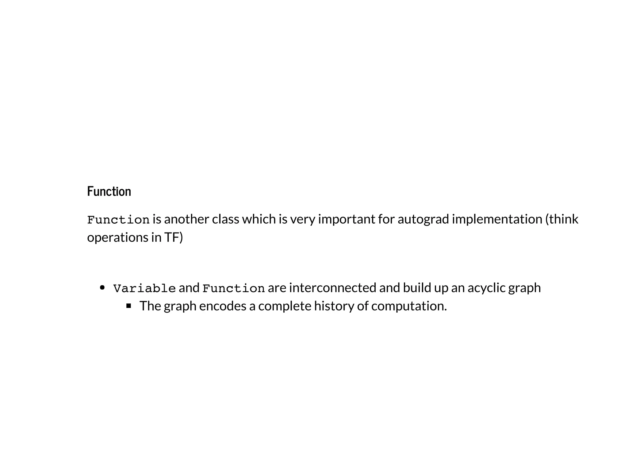
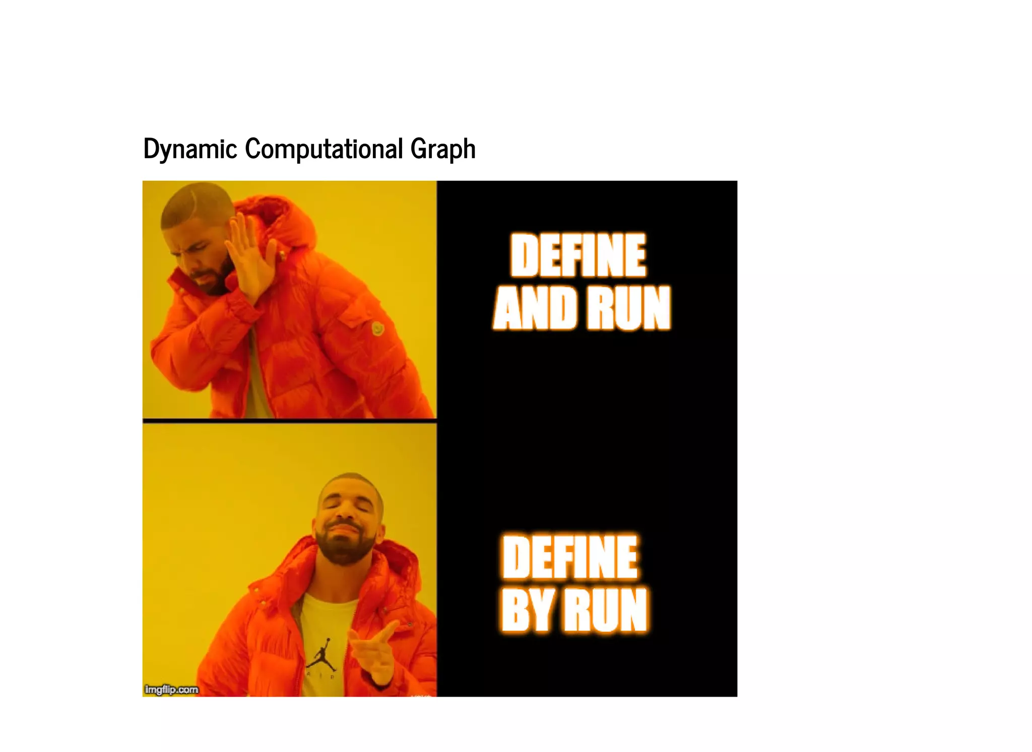
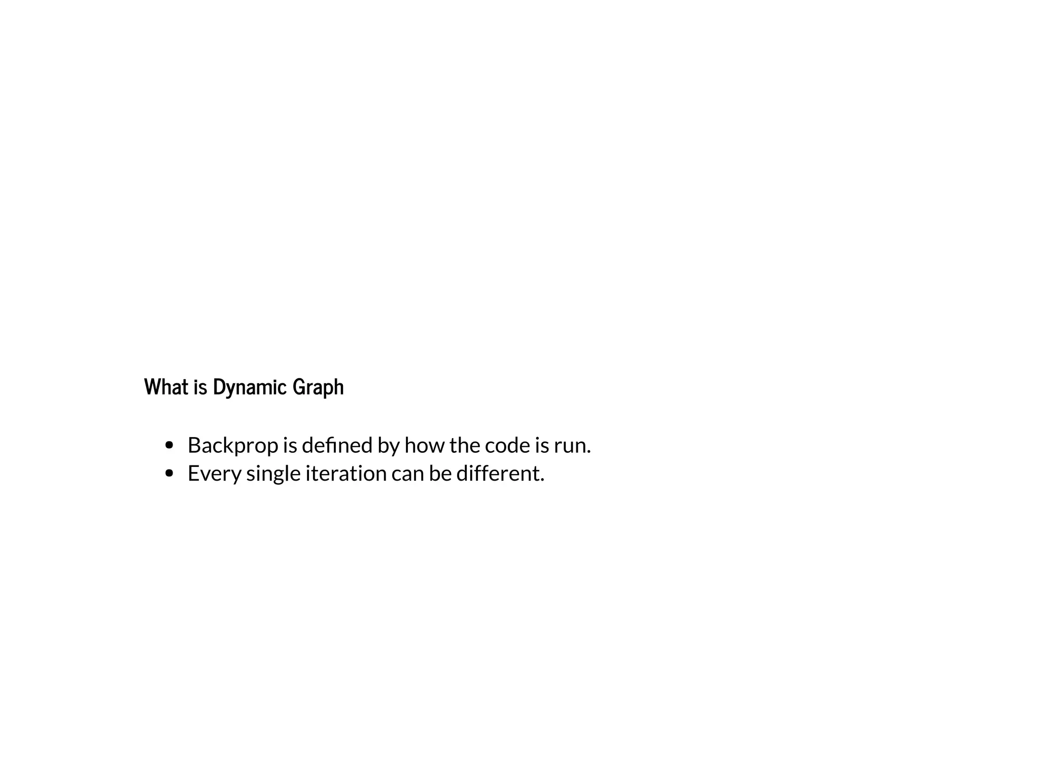
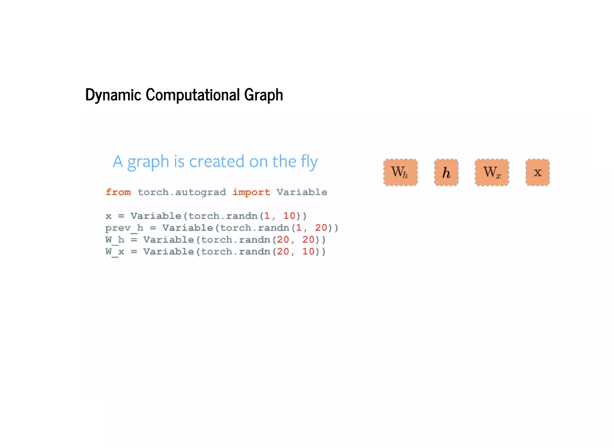
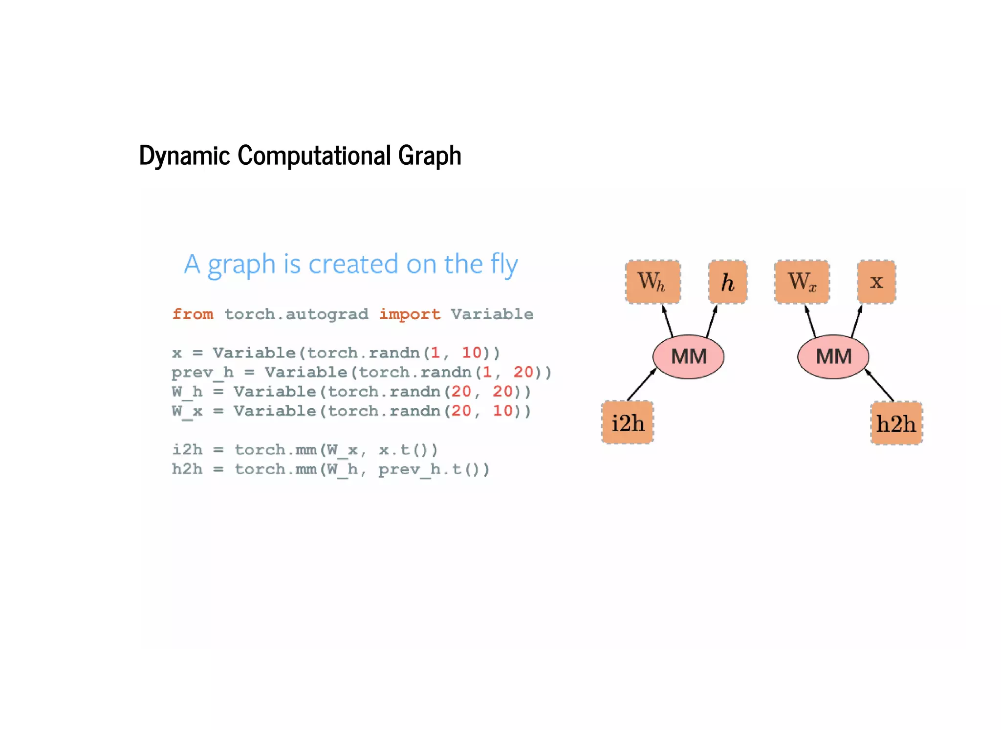
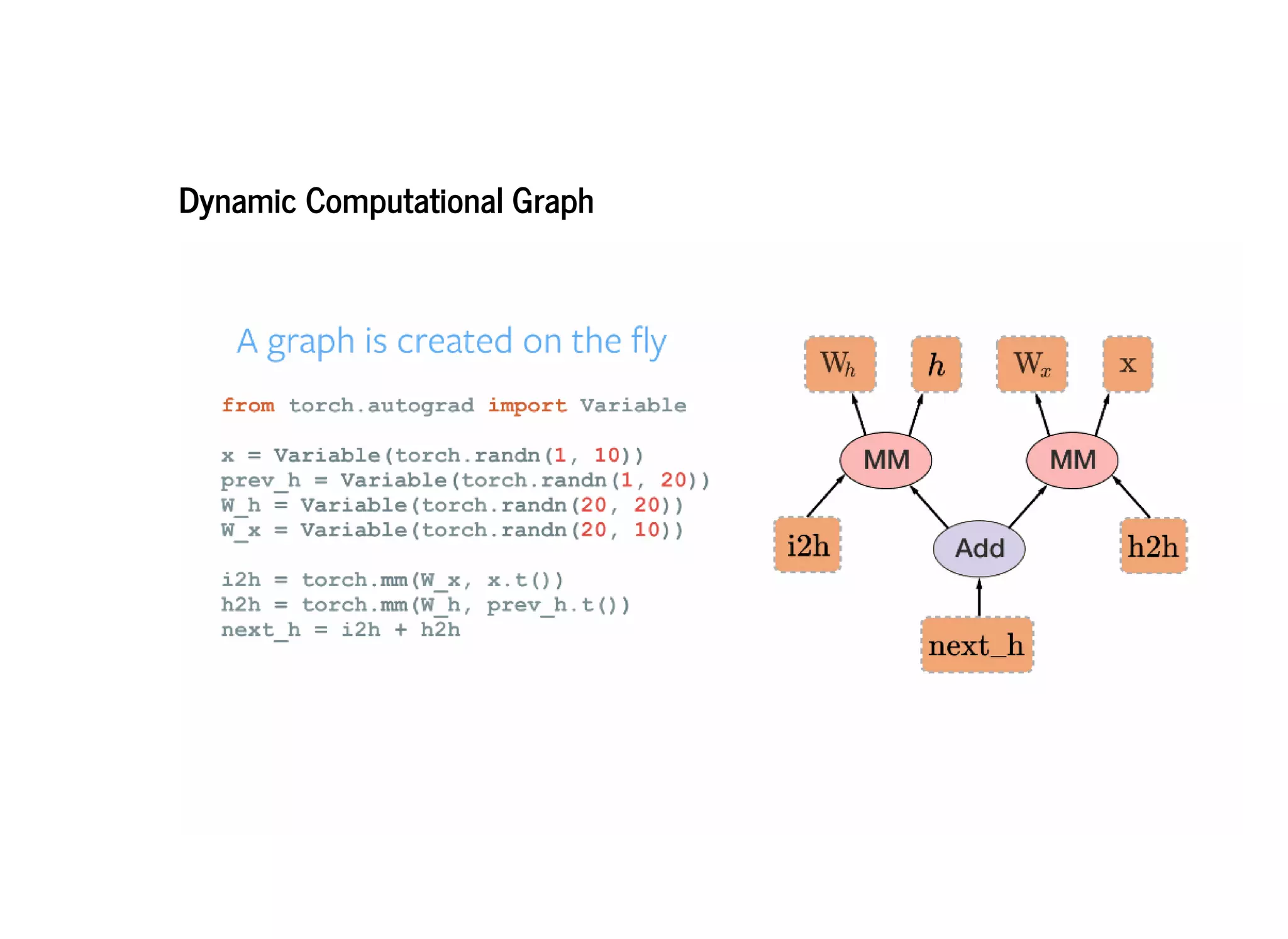
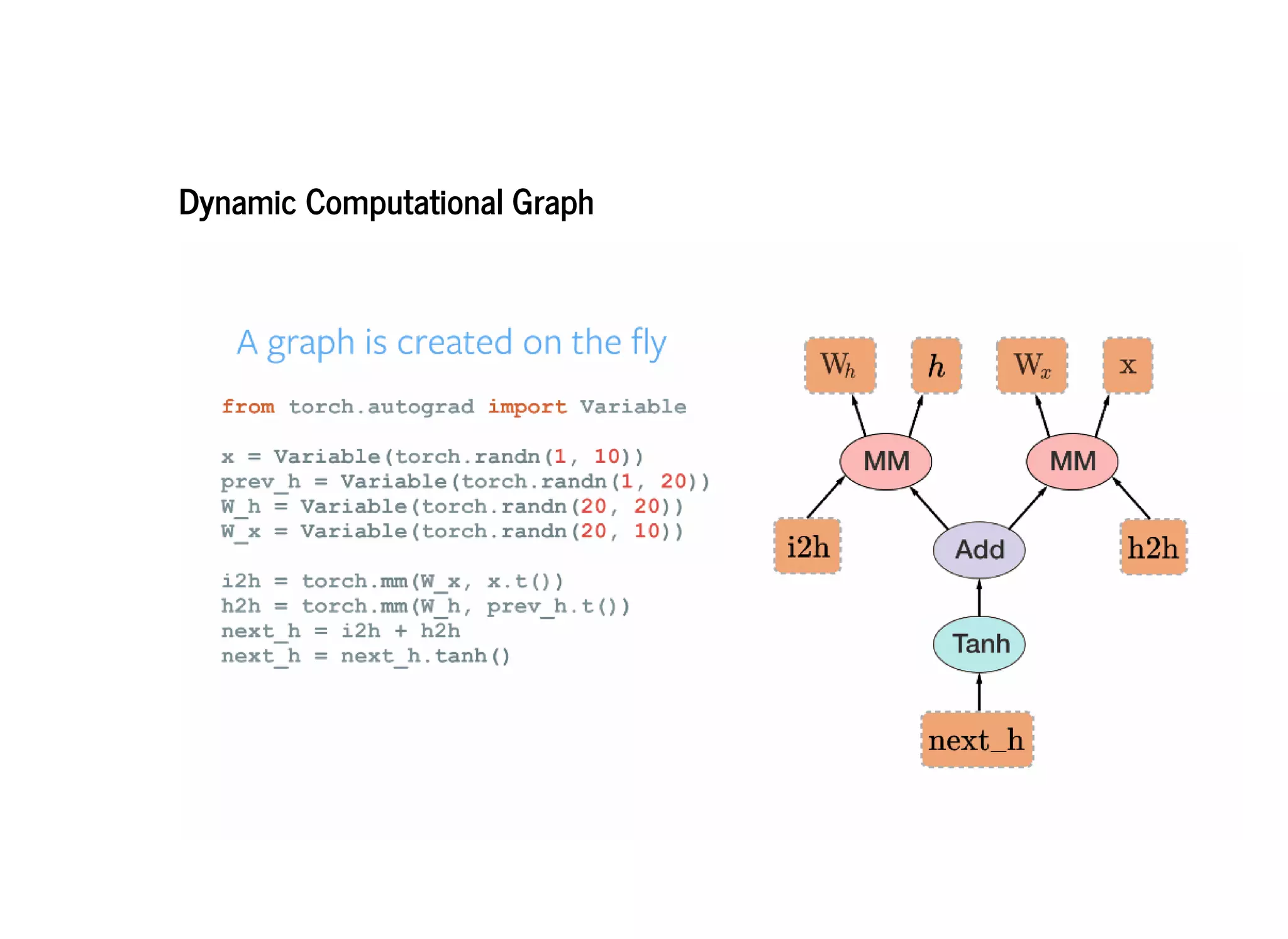
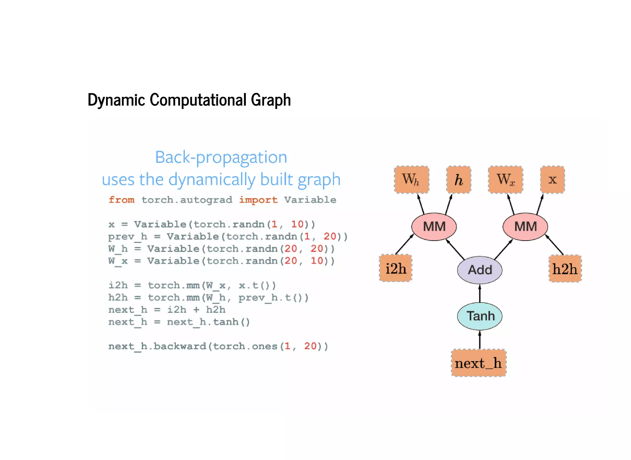
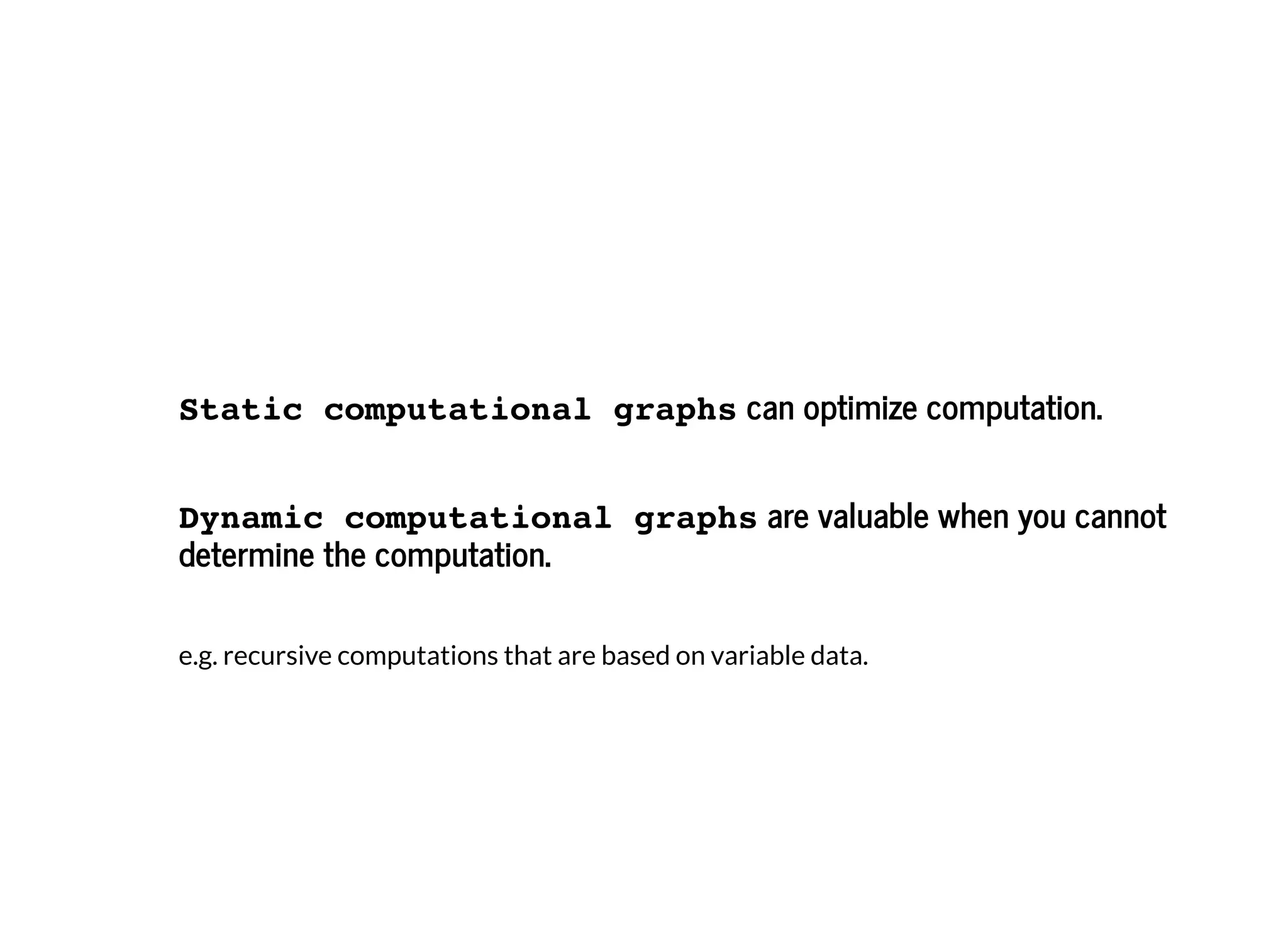
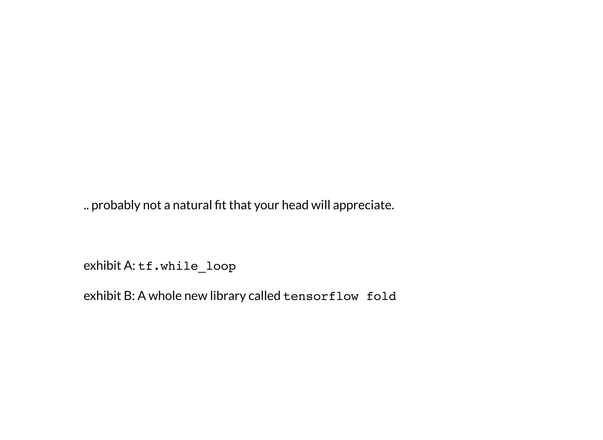
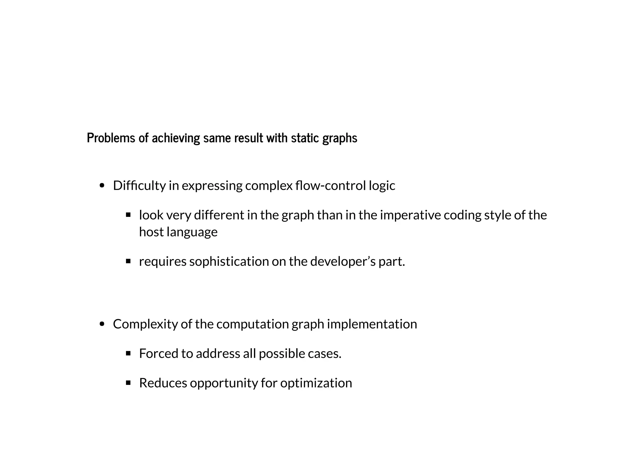
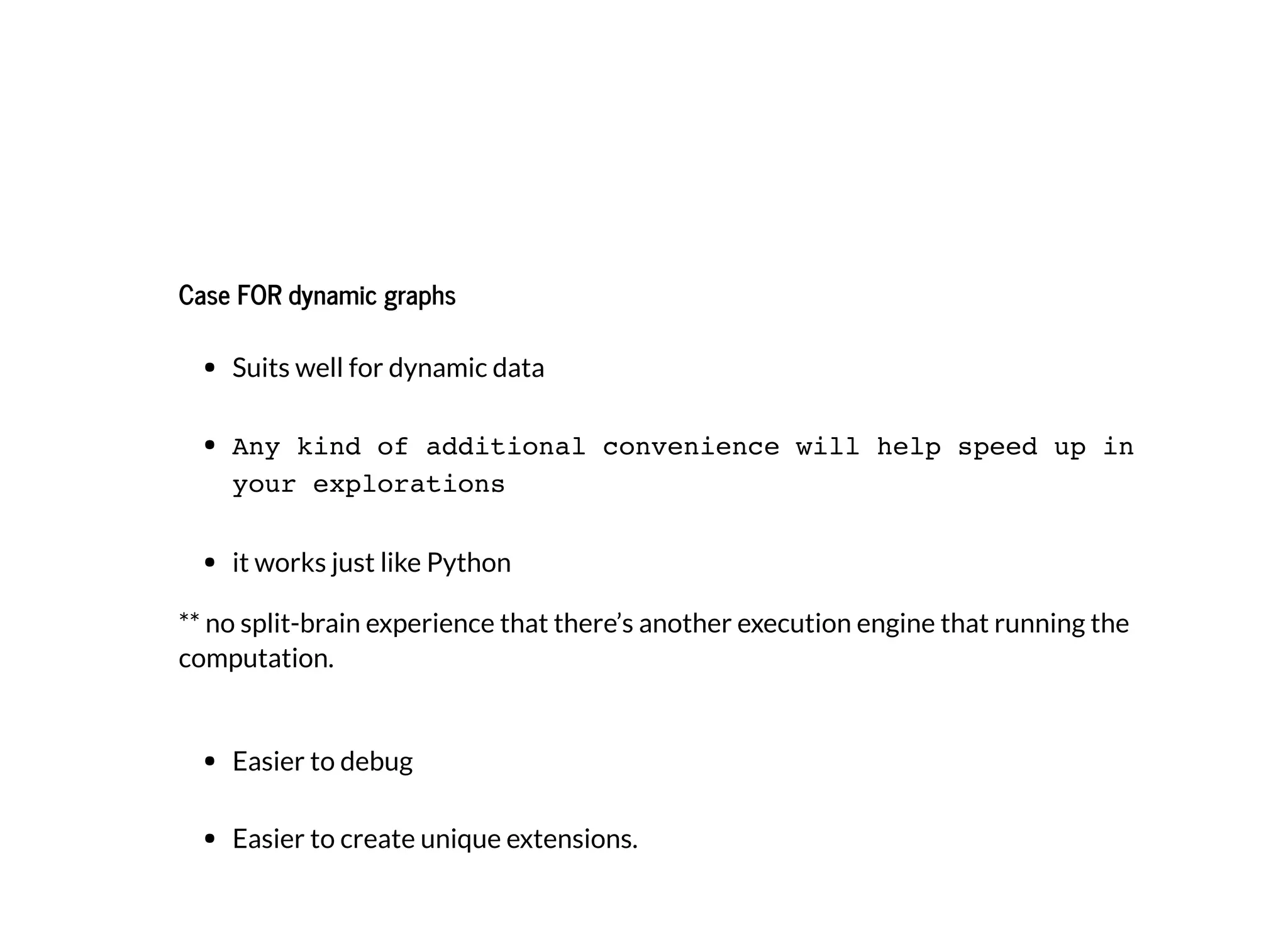
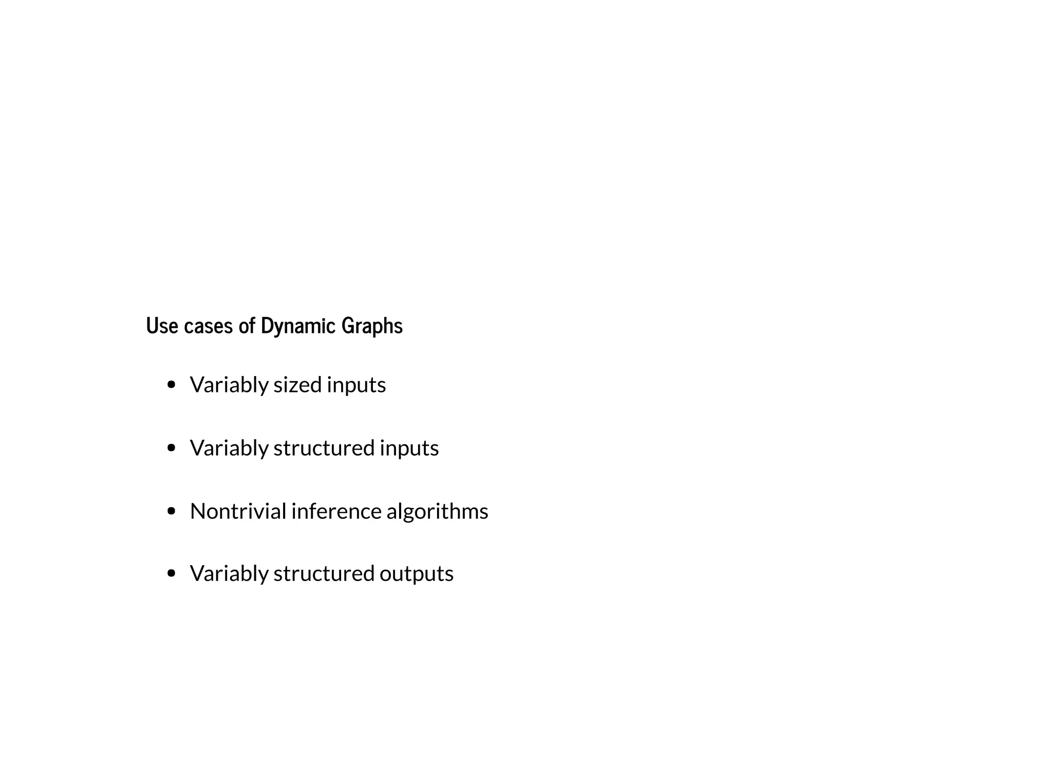
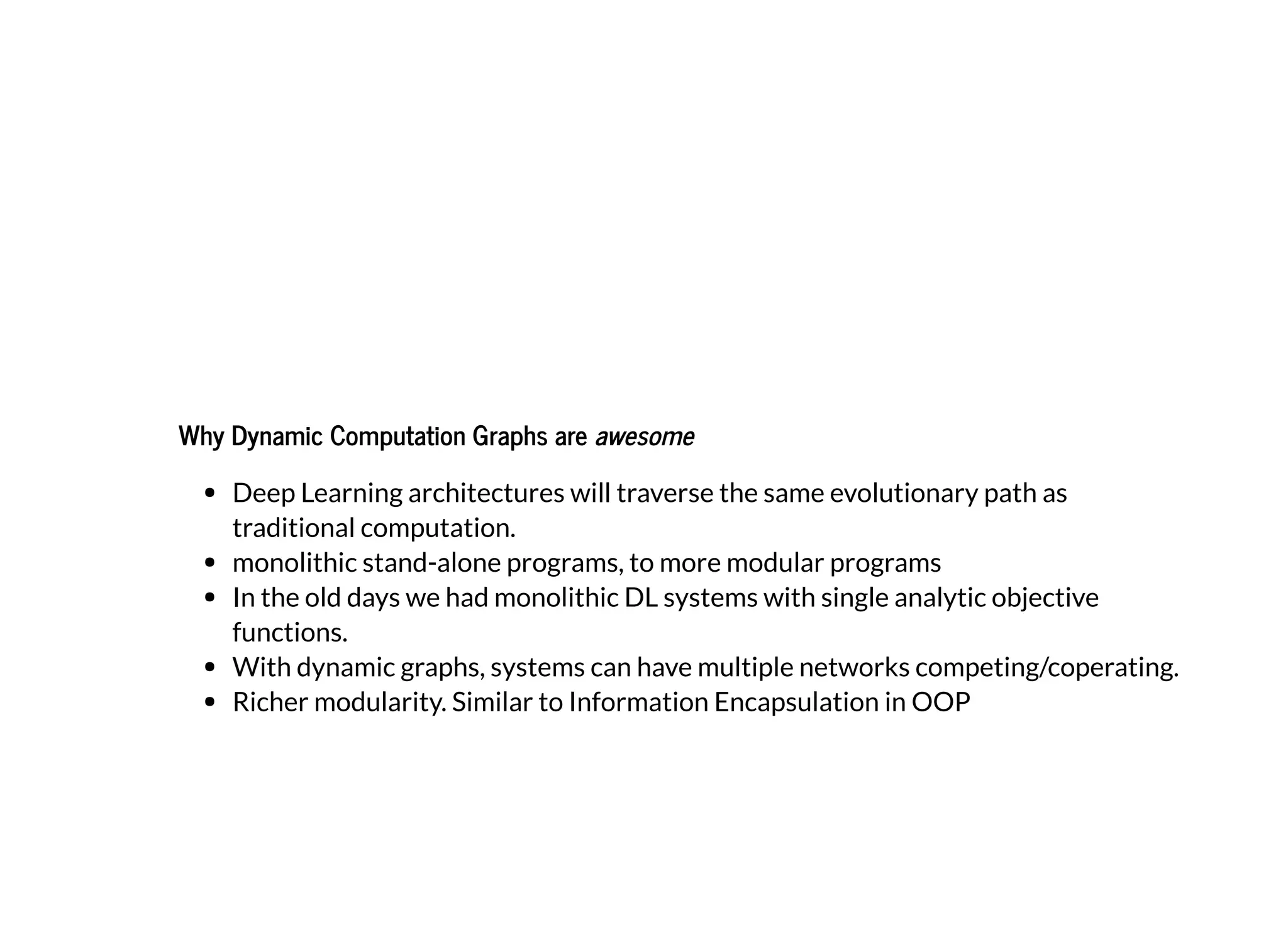
PyTorch constructs dynamic computational graphs that allow for maximum flexibility and speed for deep learning research. Dynamic graphs are useful when the computation cannot be fully determined ahead of time, as they allow the graph to change on each iteration based on variable data. This makes PyTorch well-suited for problems with dynamic or variable sized inputs. While static graphs can optimize computation, dynamic graphs are easier to debug and create extensions for. PyTorch aims to be a simple and intuitive platform for neural network programming and research.


![[Update] PyTorch Tutorial for NTU Machine Learing Course 2017](https://cdn.slidesharecdn.com/ss_thumbnails/pytorchtutorial-2017-1103-171103060015-thumbnail.jpg?width=640&height=640&fit=bounds)