Python as number crunching code glue

Python as number
crunching glue

Jiahao Chen
jiahao@mit.edu
@mitpostdoc
theochem.mit.edu

1
Thursday, September 22, 2011

This is not a crash course on scientific
computing or numerical linear algebra
Recommended texts:

nr.com

2

NumPy and SciPy
How to say:

NumPy: no official pronunciation

SciPy: “sigh pie”

3

NumPy and SciPy
How to say:

NumPy: no official pronunciation

SciPy: “sigh pie”
Where to get:

scipy.org, numpy.scipy.org

You might already have it

Otherwise, have fun installing it ;)
3

You may already know how to use numpy/
scipy!

Similar to Matlab, Octave, Scilab, R.

see:
http://mathesaurus.sourceforge.net/

In many cases, Matlab/Octave/Scilab code
can be translated easily to use numpy
+scipy+matplotlib.

Other interfaces exist: e.g. mlabwrap lets
you wrap Python around Matlab.
4

Approximately continuous arithmetic
floating point*

- vs -

Exact discrete arithmetic
booleans, integers, strings, ...

*David Goldberg, “What every computer scientist should know
about floating-point arithmetic”

5

Using numpy can make code cleaner

import numpy as np
a = range(10000000) a = np.arange(10000000)
b = range(10000000) b = np.arange(10000000)
c = [] c = a + b

for i in range(len(a)):
c.append(a[i] + b[i])

What’s different??

6

What’s different?creates list of creates ndarray of
dynamically typed int statically typed int
import numpy as np
a = range(10000000) a = np.arange(10000000)
b = range(10000000) b = np.arange(10000000)
c = [] #a+b is concatenation c = a + b #vectorized addition

for i in range(len(a)):
c.append(a[i] + b[i])

Using numpy can save lots of time

7.050s 0.333s (21x)
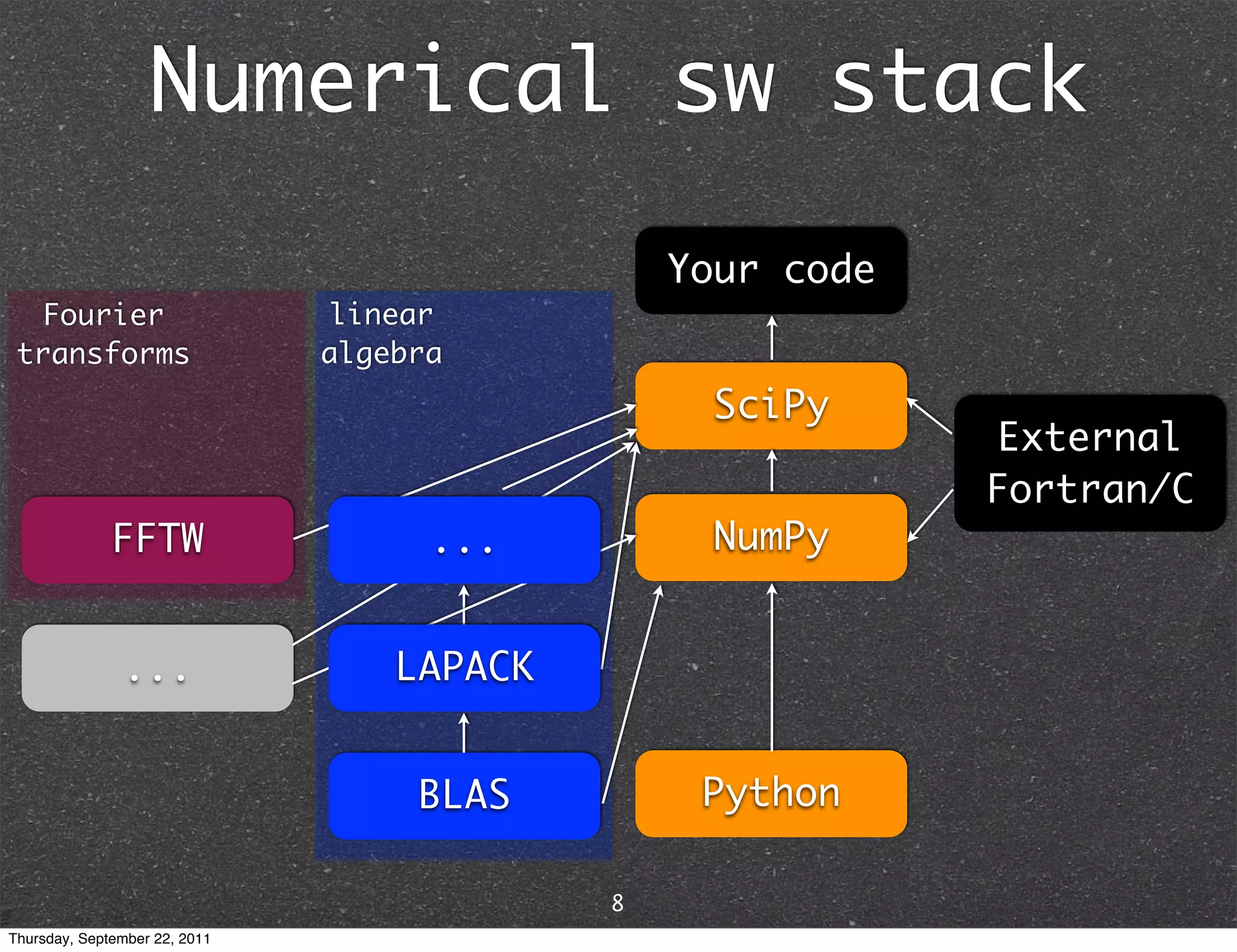
a convenient interface to compiled C/Fortran
libraries: BLAS, LAPACK, FFTW, UMFPACK,...

7

Numerical sw stack
Your code
Fourier linear
transforms algebra
SciPy
External
Fortran/C
FFTW ... NumPy

... LAPACK

BLAS Python

8

“One thing that graduate students eventually
learn is that you can hide just about
anything in a NxN matrix... (for sufficiently
large N)” - anonymous string theorist

9

“One thing that graduate students eventually
learn is that you can hide just about
anything in a NxN matrix... (for sufficiently
large N)” - anonymous string theorist

If your data can be put into a matrix/vector,
numpy/scipy can help you!

9

You may already be working with matrix/vector
data...

bitmap/video waveform graph

database differential
text
table equation model
10

# Chapter NumPy SciPy

1 Scientific Computing
2 Systems of linear equations X X

3 Linear least squares X

4 Eigenvalue problems X X

5 Nonlinear equations X

6 Optimization X

7 Interpolation X

8 Numerical integration and differntiation X

9 Initial value problems for ODEs X

10 Boundary value problems for ODEs X

11 Partial differential equations X

12 Fast Fourier Transform X

13 Random numbers and stochastic simulation X

Table of contents from Michael Heath’s textbook
11

Outline:

* NumPy: explicit data typing with dtypes
: array manipulation with ndarrays

* SciPy: high-level numerical routines
: use cases

* NumPy/SciPy as code glue: f2py and weave

12

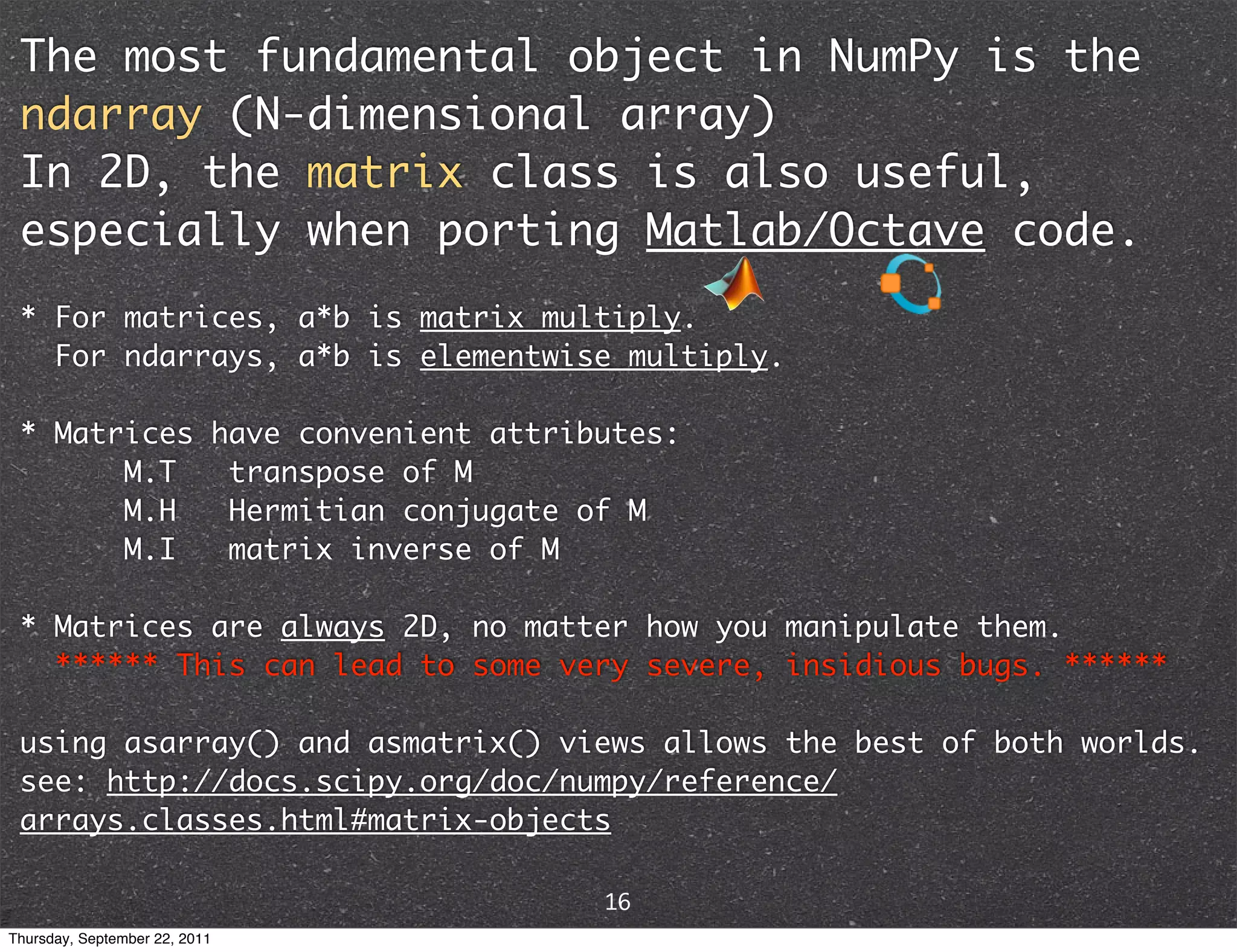
The most fundamental object in NumPy is the
ndarray (N-dimensional array)

v[:] vector
M[:,:] matrix
x[:,:,...,:] higher order tensor

unlike built-in Python data types,
ndarrays are designed for
homogeneous, explicitly typed data

13

numpy primitive dtypes
Signed Unsigned
Bits Boolean Float Complex
integer integer
8 bool int8 uint8
16 int16 uint16
32 int32 uint32 float32
int intp uint float
64 complex64
int64 uint64 float64
128 float128 complex128
256 complex256

dtypes bring explicit typing to Python

14

Structured array: ndarray of data structure

>>> mol = np.zeros(3, dtype=('uint8, 3float64'))
>>> mol[0] = 8, (-0.464, 0.177, 0.0)
>>> mol[1] = 1, (-0.464, 1.137, 0.0)
>>> mol[2] = 1, (0.441, -0.143, 0.0)
>>> mol
array([(8, [-0.46400000000000002, 0.17699999999999999, 0.0]),
(1, [-0.46400000000000002, 1.137, 0.0]),
(1, [0.441, -0.14299999999999999, 0.0])],
dtype=[('f0', '|u1'), ('f1', '<f8', (3,))])

Recarray: ndarray of data structure
with named fields (record)
>>> mol = np.array(mol,
dtype={'atomicnum':('uint8',0), 'coords':('3float64',1)})
>>> mol['atomicnum']
array([8, 1, 1], dtype=uint8)

15

The most fundamental object in NumPy is the
ndarray (N-dimensional array)
In 2D, the matrix class is also useful,
especially when porting Matlab/Octave code.
* For matrices, a*b is matrix multiply.
For ndarrays, a*b is elementwise multiply.

* Matrices have convenient attributes:
M.T transpose of M
M.H Hermitian conjugate of M
M.I matrix inverse of M

* Matrices are always 2D, no matter how you manipulate them.
****** This can lead to some very severe, insidious bugs. ******

using asarray() and asmatrix() views allows the best of both worlds.
see: http://docs.scipy.org/doc/numpy/reference/
arrays.classes.html#matrix-objects

16

Memory layout of
matrices
column major: first dimension is
contiguous in memory
Fortran, Matlab, R,...

row major: last dimension is
contiguous in memory
C, Java, numpy,...

Why you should care:
• Cache coherence
• Transposing a matrix is very expensive
17

Creating ndarrays
• from Python iterable: lists, tuples,...
e.g. array([1, 2, 3]) == asarray((1, 2, 3))
• from intrinsic functions
empty() allocates memory only
zeros() initializes to 0
ones() initializes to 1
arange() creates a uniform range
rand() initializes to uniform random
randn() initializes to standard normal random
...
• from binary representation in string/buffer
• from file on disk
18

Generating ndarrays
fromfunction() creates an ndarray whose
entries are functions of its indices

e.g. the Hilbert matrix

1..n
>>> np.fromfunction(lambda i,j: 1./(i+j+1), (4,4))
array([[ 1. , 0.5 , 0.33333333, 0.25 ],
[ 0.5 , 0.33333333, 0.25 , 0.2 ],
[ 0.33333333, 0.25 , 0.2 , 0.16666667],
[ 0.25 , 0.2 , 0.16666667, 0.14285714]])

19

Generating ndarrays
arange(): like range() but accepts floats
>>> import numpy as np
>>> np.arange(2, 2.5, 0.1)
array([ 2. , 2.1, 2.2, 2.3, 2.4])

linspace(): creates array with speciﬁed
number of elements, spaced equally between
the speciﬁed beginning and ending.
>>> np.linspace(2.0, 2.4, 5)
array([ 2. , 2.1, 2.2, 2.3, 2.4])

20

ndarray native I/O
Format Reader Writer
pickle.loads()
pickle dumps()

NPY np.load() np.save()
NPZ np.savez()
Memory map np.memmap

NPY is numpy’s native binary format
NPZ is a zip file of NPYs
Memory map: a class useful for handling huge matrices
won’t load entire matrix into memory

21

ndarray text I/O
eval() np.array_repr()
String
or below with StringIO
np.loadtxt()
Text file np.genfromtxt() savetxt()
np.recfromtxt()
CSV np.recfromcsv()
Matrix
scipy.io.mmread() mmwrite()
Market

22

ndarray binary I/O
List np.array() ndarray.tolist()
np.fromstring() tostring()
String
or below with StringIO
Raw binary scipy.io.numpyio.fread() fwrite()
file ndarray.fromfile() .tofile()
MATLAB scipy.io.loadmat() savemat()
netCDF scipy.io.netcdf.netcdf_file
WAV audio scipy.io.wavfile.read() write()
Image scipy.misc.imread() imsave()
(via PIL) scipy.misc.fromimage() toimage()
Also video (OpenCV), HDF5 (PyTables), FITS (PyFITS)...
23

Indexing
>>> x = np.arange(12).reshape(3,4); x
array([[ 0, 1, 2, 3],
[ 4, 5, 6, 7],
[ 8, 9, 10, 11]])
>>> x[1,2]
6
>>> x[2,-1] row, then column
11
>>> x[0][2]
2
>>> x[(2,2)] #tuple
10
>>> x[:1] #slices return views, not copies
array([[0, 1, 2, 3]])
>>> x[::2,1:4:2]
array([[ 1, 3],
[ 9, 11]])

24

Fancy indexing
>>> x = np.arange(12).reshape(3,4); x
array([[ 0, 1, 2, 3],
[ 4, 5, 6, 7],
[ 8, 9, 10, 11]])
>>> x[(2,2)]
array index
10
>>> x[np.array([2,2])] #same as x[[2,2]]
array([[ 8, 9, 10, 11],
[ 8, 9, 10, 11]])
>>> x[np.array([1,0]), np.array([2,1])]
array([6, 1])
>>> x[x>8] Boolean mask
array([ 9, 10, 11])
>>> x>8
array([[False, False, False, False],
[False, False, False, False],
[False, True, True, True]], dtype=bool)

25

Fancy indexing II
>>> y = np.arange(1*2*3*4).reshape(1,2,3,4); y
array([[[[ 0, 1, 2, 3],
[ 4, 5, 6, 7],
[ 8, 9, 10, 11]],

[[12, 13, 14, 15],
[16, 17, 18, 19],
[20, 21, 22, 23]]]])

>>> y[0, Ellipsis, 0] # == y[0, ..., 0] == [0,:,:,0]
array([[ 0, 4, 8],
[12, 16, 20]])
>>> y[0, 0, 0, slice(2,4)] # == y[(0, 0, 0, 2:4)]
array([2, 3])

26

Broadcasting
What happens when you multiply ndarrays of
different dimensions?

Case I: trailing dimensions match
>>> x #.shape = (3,4)
array([[ 0, 1, 2, 3],
>>> y * x
[ 4, 5, 6, 7],
array([[[[ 0, 1, 4, 9],
[ 8, 9, 10, 11]])
[ 16, 25, 36, 49],
>>> y #.shape = (1,2,3,4)
[ 64, 81, 100, 121]],
array([[[[ 0, 1, 2, 3],
[ 4, 5, 6, 7],
[[ 0, 13, 28, 45],
[ 8, 9, 10, 11]],
[ 64, 85, 108, 133],
[160, 189, 220, 253]]]])
[[12, 13, 14, 15],
[16, 17, 18, 19],
[20, 21, 22, 23]]]])

27

Broadcasting
What happens when you multiply ndarrays of
different dimensions?

Case II: trailing dimension is 1
>>> b.shape = 4,1
>>> a + b
>>> a = np.arange(4); a array([[3, 4, 5, 6],
array([0, 1, 2, 3]) [2, 3, 4, 5],
>>> b = np.arange(4)[::-1]; b [1, 2, 3, 4],
array([3, 2, 1, 0]) [0, 1, 2, 3]])
>>> a + b
array([3, 3, 3, 3])
>>> b.shape = 1,4
>>> a + b
array([[3, 3, 3, 3]])

28

Matrix operations
In 2D, the matrix class is often more useful
than ndarrays, especially when porting
Matlab/Octave code.
* For matrices, a*b is matrix multiply.
For ndarrays, a*b is elementwise multiply.

* Matrices have convenient attributes:
M.T transpose of M
M.H Hermitian conjugate of M
M.I matrix inverse of M

* Matrices are always 2D, no matter how you manipulate them.
****** This can lead to some very severe, insidious bugs. ******

using asarray() and asmatrix() views allows the best of both worlds.
see: http://docs.scipy.org/doc/numpy/reference/
arrays.classes.html#matrix-objects
29

Matrix functions
You can apply a function elementwise to a
matrix...
>>> from numpy import array, exp
>>> X = array([[1, 1], [1, 0]])
>>> exp(X)
array([[ 2.71828183, 2.71828183],
[ 2.71828183, 1.]])

...or a matrix version of that function
>>> from scipy.linalg import expm
>>> expm(X)
array([[ 2.71828183, 7.3890561 ],
[ 1. , 2.71828183]])

other functions in scipy.linalg.matfuncs
30

SciPy by example

* Data fitting

* Signal matching

* Disease outbreak modeling (epidemiology)

http://scipy-central.org/
31

Least-squares curve fitting
from scipy import *
fit data to model from scipy.optimize import leastsq
from matplotlib.pyplot import plot

#Make up data x(t) with Gaussian noise
num_points = 150
t = linspace(5, 8, num_points)
x = 11.86*cos(2*pi/0.81*t-1.32) + 0.64*t
+4*((0.5-rand(num_points))*
exp(2*rand(num_points)**2))

# Target function
model = lambda p, x:
p[0]*cos(2*pi/p[1]*x+p[2]) + p[3]*x
# Distance to the target function
error = lambda p, x, y: model(p, x) - y
# Initial guess for the parameters
p0 = [-15., 0.8, 0., -1.]
p1, _ = leastsq(error, p0, args=(t, x))

t2 = linspace(t.min(), t.max(), 100)
plot(t, x, "ro", t2, model(p1, t2), "b-")
raw_input()

32

Matching signals
Suppose I have a short audio clip

that I know to be part of a larger file

How can I figure out its offset?

Problem: naïve matching scales as O(N2)

33

An O(N lg N) solution
Naïve matching scales as O(N2)
How can we do faster?

phase correlation

Exploit Fourier transforms: they encode
relative offsets in complex phase

60o

1/6 34

From math to code

35

From math to code
import numpy

#Make up some data
N = 30000
idx = 24700
size = 300
data = numpy.random.rand(N)
frag_pad = numpy.zeros(N)
frag = data[idx:idx+size]
frag_pad[:size] = frag

#Compute phase correlation
data_ft = numpy.fft.rfft(data)
frag_ft = numpy.fft.rfft(frag_pad)
phase = data_ft * numpy.conj(frag_ft)
phase /= abs(phase)
cross_correlation = numpy.fft.irfft(phase)
offset = numpy.argmax(cross_correlation)

print 'Input offset: %d, computed: %d' % (idx, offset)
from matplotlib.pyplot import plot
plot(cross_correlation)
raw_input() #Pause

35

Modeling a zombie apocalypse

http://blogs.cdc.gov/publichealthmatters/2011/05/preparedness-101-
zombie-apocalypse/

36

Each person can be in one of three states

Normal (S) Zombie Dead (R)

http://www.scipy.org/Cookbook/Zombie_Apocalypse_ODEINT

37

transmission (B) resurrection (G)

Normal (S) Zombie Dead (R)
+
destruction (A)
birth (P) normal death
Various processes connect these states

38

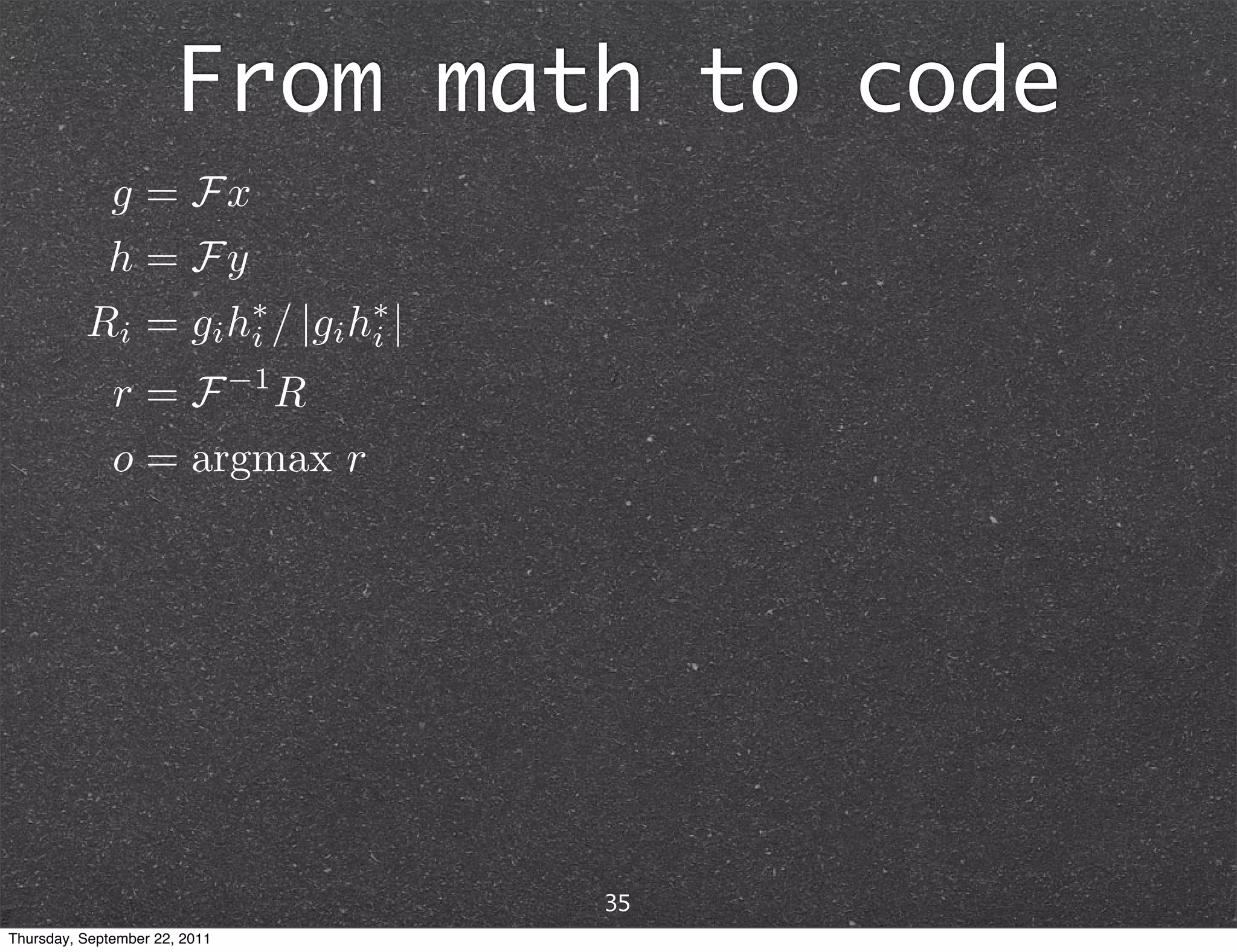
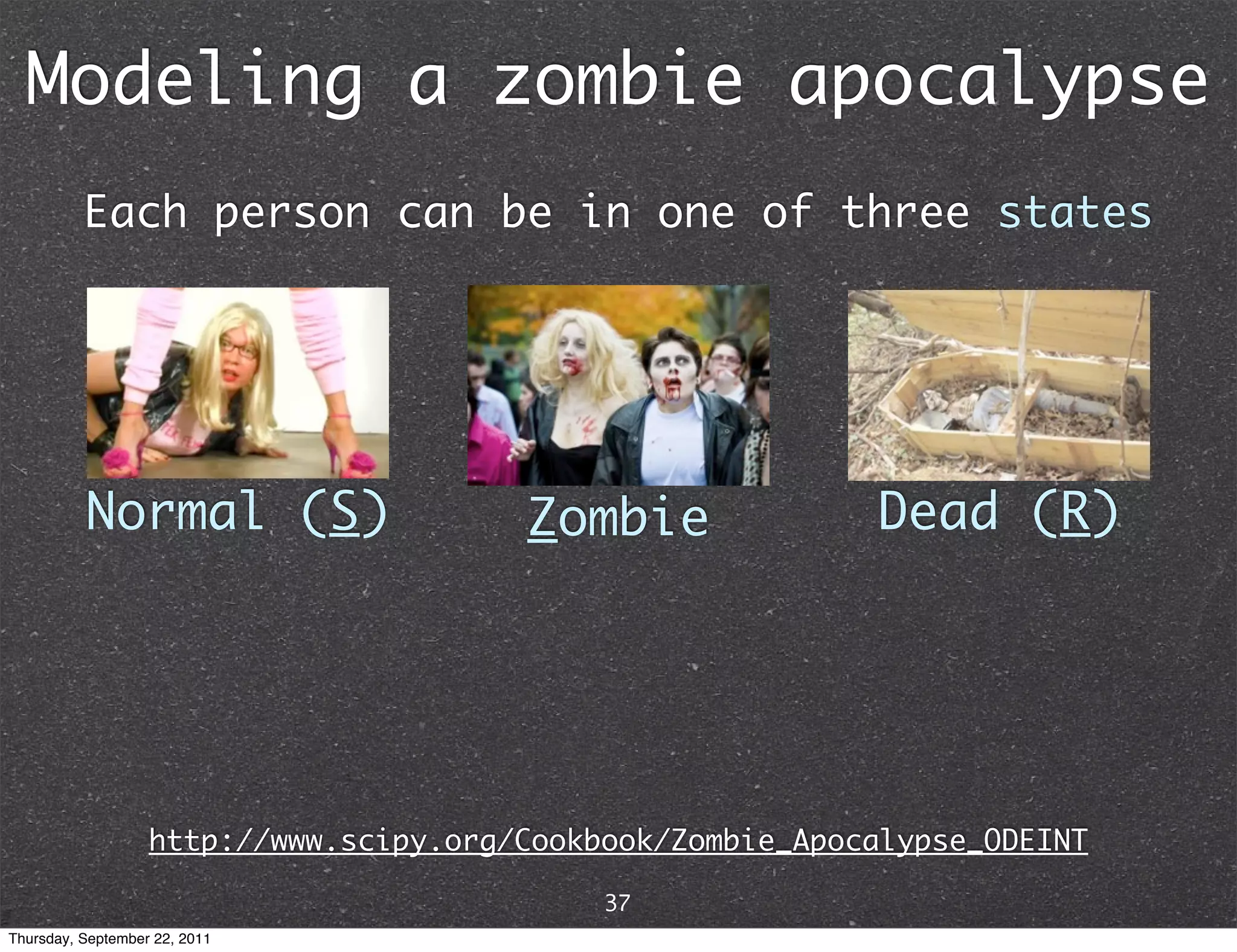
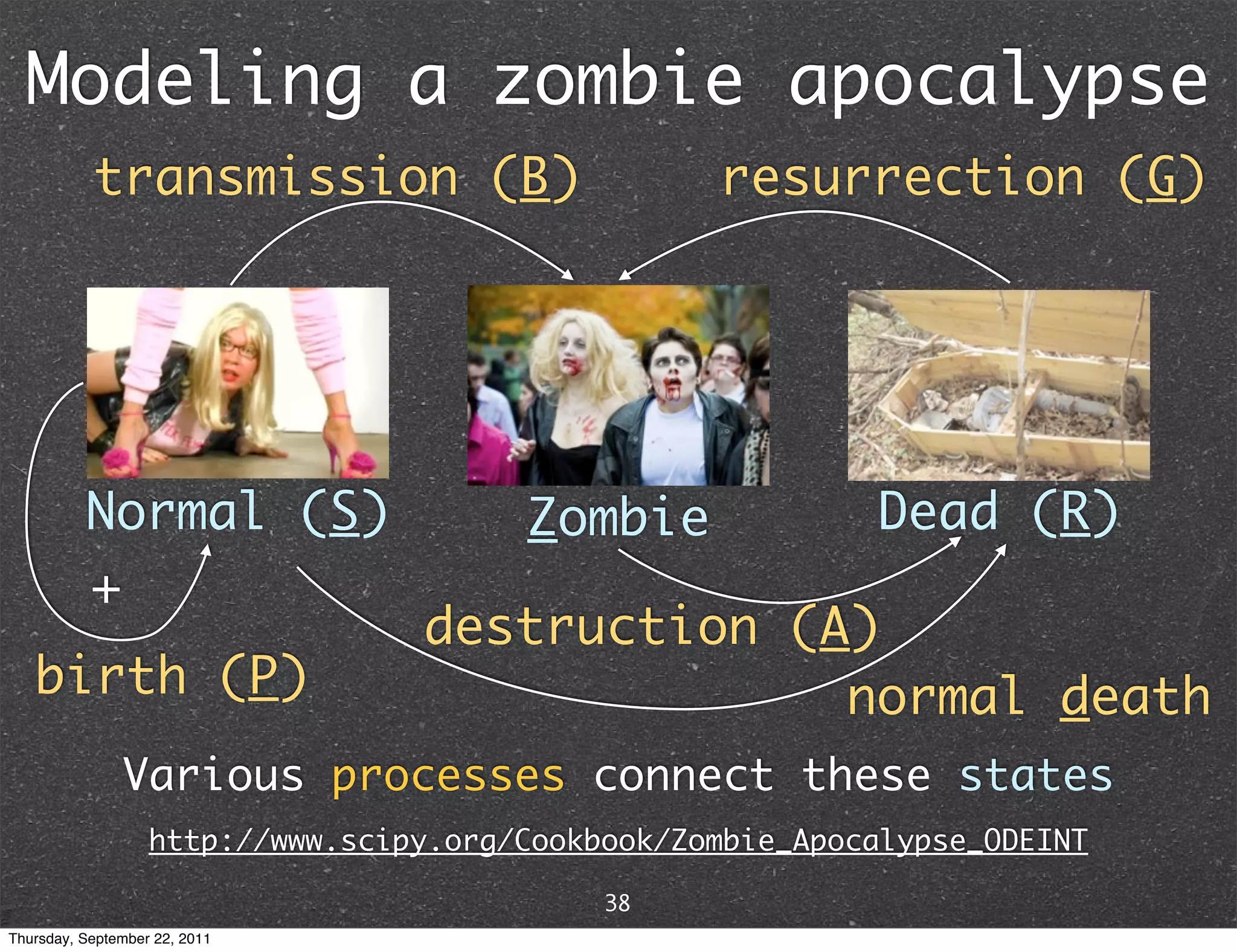
From math to code
B G from numpy import linspace
from scipy.integrate import odeint

P = 0 # birth rate
d = 0.0001 # natural death rate
S Z R B = 0.0095 # transmission rate
+ A G = 0.0001 # resurrection rate
A = 0.0001 # destruction rate
r d def f(y, t):
Si, Zi, Ri = y
return [P - B*Si*Zi - d*Si,
B*Si*Zi + G*Ri - A*Si*Zi,
d*Si + A*Si*Zi - G*Ri]

y0 = [500, 0, 0] # initial conditions
t = linspace(0, 5., 1000) # time grid

soln = odeint(f, y0, t) # solve ODE
S, Z, R = soln[:, :].T


39

Using external code
“NumPy can get you most of the way to compiled speeds through
vectorization. In situations where you still need the last ounce
of speed in a critical section, or when it either requires a PhD
in NumPy-ology to vectorize the solution or it results in too
much memory overhead, you can reach for Cython or Weave. If you
already know C/C++, then weave is a simple and speedy solution.
If, however, you are not already familiar with C then you may
find Cython to be exactly what you are looking for to get the
speed you need out of Python.” - Travis Oliphant, 2011-06-20

see:
http://www.scipy.org/PerformancePython
http://technicaldiscovery.blogspot.com/
2011/06/speeding-up-python-numpy-cython-
and.html
40

Python as code glue
- numpy.f2py: wraps
* C, Fortran 77/90/95 functions
* Fortran 90/95 module data
* Fortran 77 COMMON blocks

- scipy.weave
* .inline: compiles & runs C/C++ code
manipulating Python scalars/ndarrays
* .blitz: interfaces with Blitz++

Other wrapper libraries and programs: see
http://scipy.org/Topical_Software
41

numpy.f2py: Fortran/C
$ cat>invsqrt.c
#include <math.h>
double invsqrt(a) {
$ cat>invsqrt.f
return 1.0/sqrt(a);
real*8 function invsqrt (a)
}
real*8 a
$ cat>invsqrt.m
invsqrt = 1.0/sqrt(a)
python module invsqrt
end
interface
real*8 function invsqrt(x)
$ f2py -c -m invsqrt invsqrt.f
intent(c) :: invsqrt
$ python -c 'import invsqrt;
real*8 intent(in) :: x
print invsqrt.invsqrt(4)'
end function invsqrt
0.5
end interface
end python module invsqrt
see: http://www.scipy.org/F2py
$ f2py invsqrt.m invsqrt.c -c
$ python -c 'import invsqrt;
print invsqrt.invsqrt(4)'
0.5
42

scipy.weave.inline
python on-the-fly
scipy distutils compiled
weave core C/C++
program
inline Extension

>>> from scipy.weave import inline
>>> x = 4.0
>>> inline('return_val = 1./sqrt(x));',
['x'])
0.5

see: https://github.com/scipy/scipy/blob/
master/scipy/weave/doc/tutorial.txt
43

scipy.weave.blitz
Uses the Blitz++ numerical library for C++
Converts between ndarrays and Blitz arrays
>>> # Computes five-point average using numpy and weave.blitz
>>> import numpy import empty
>>> from scipy.weave import blitz
>>> a = numpy.zeros((4096,4096)); c = numpy.zeros((4096, 4096))
>>> b = numpy.random.randn(4096,4096)
>>> c[1:-1,1:-1] = (b[1:-1,1:-1] + b[2:,1:-1] + b[:-2,1:-1] + b
[1:-1,2:] + b[1:-1,:-2]) / 5.0
>>> blitz("a[1:-1,1:-1] = (b[1:-1,1:-1] + b[2:,1:-1] + b
[:-2,1:-1] + b[1:-1,2:] + b[1:-1,:-2]) / 5.")
>>> (a == c).all()
True

see:
https://github.com/scipy/scipy/blob/master/scipy/weave/doc/
tutorial.txt
44

Parallelization
The easy way: numpy/scipy’s primitives
automatically use vectorization compiled
into external BLAS/LAPACK/... libraries

The usual way:
- MPI interfaces (mpi4py,...)
- Python threads/multiprocessing/...
- OpenMP/pthreads... in external C/Fortran

see:
http://www.scipy.org/ParallelProgramming

45

How I use NumPy/Scipy
Text External
Text input
output binary

Binary
output
scipy.optimize
ndarray. Quasi-Newton optimizers
fromfile()
Matrices Test model Visualize

46

Beyond NumPy/SciPy
My script My interactive session
visualization
HDF5 numerical plots
file I/O optimization Pylab
molecule
viz.

PyTables CVXOpt VTK matplotlib PyMol

SciPy
External
Fortran/C
NumPy

Python
many more examples at http://www.scipy.org/Topical_Software
47

Python as number crunching code glue

More Related Content

What's hot

Viewers also liked

Similar to Python as number crunching code glue

Recently uploaded

Python as number crunching code glue