Graphs and Trees
CourseCode: CSC 2211
Dept. of Computer Science
Faculty of Science and Technology
Lecturer No: Week No: 10 Semester: Spring 2019-2020
Lecturer: Name & email
Course Title: Algorithms
2.
Lecture Outline
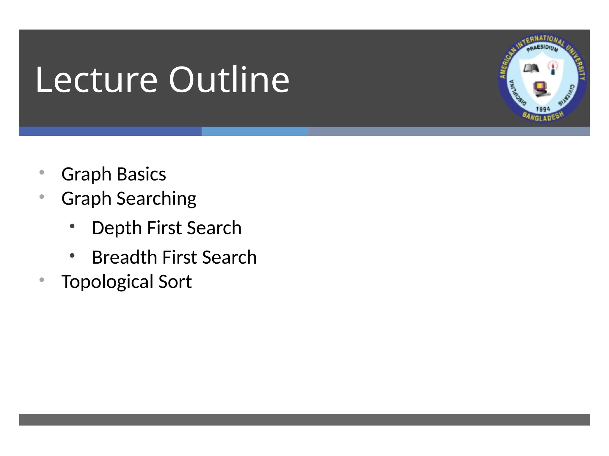
• GraphBasics
• Graph Searching
• Depth First Search
• Breadth First Search
• Topological Sort
3.
Graphs
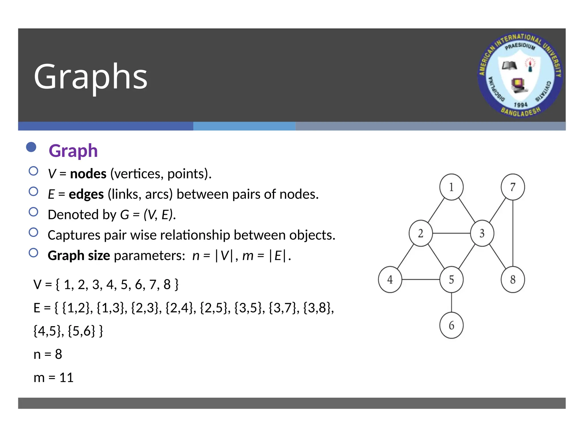
Graph –mathematical object consisting of a set of:
V = nodes (vertices, points).
E = edges (links, arcs) between pairs of nodes.
Denoted by G = (V, E).
Captures pair wise relationship between objects.
Graph size parameters: n = |V|, m = |E|.
V = { 1, 2, 3, 4, 5, 6, 7, 8 }
E = { {1,2}, {1,3}, {2,3}, {2,4}, {2,5}, {3,5}, {3,7}, {3,8},
{4,5}, {5,6} }
n = 8
m = 11
4.
Graphs
1 2
3 4
12
3 4
Directed
graph
Undirected
graph
1 2
3 4
Acyclic
graph
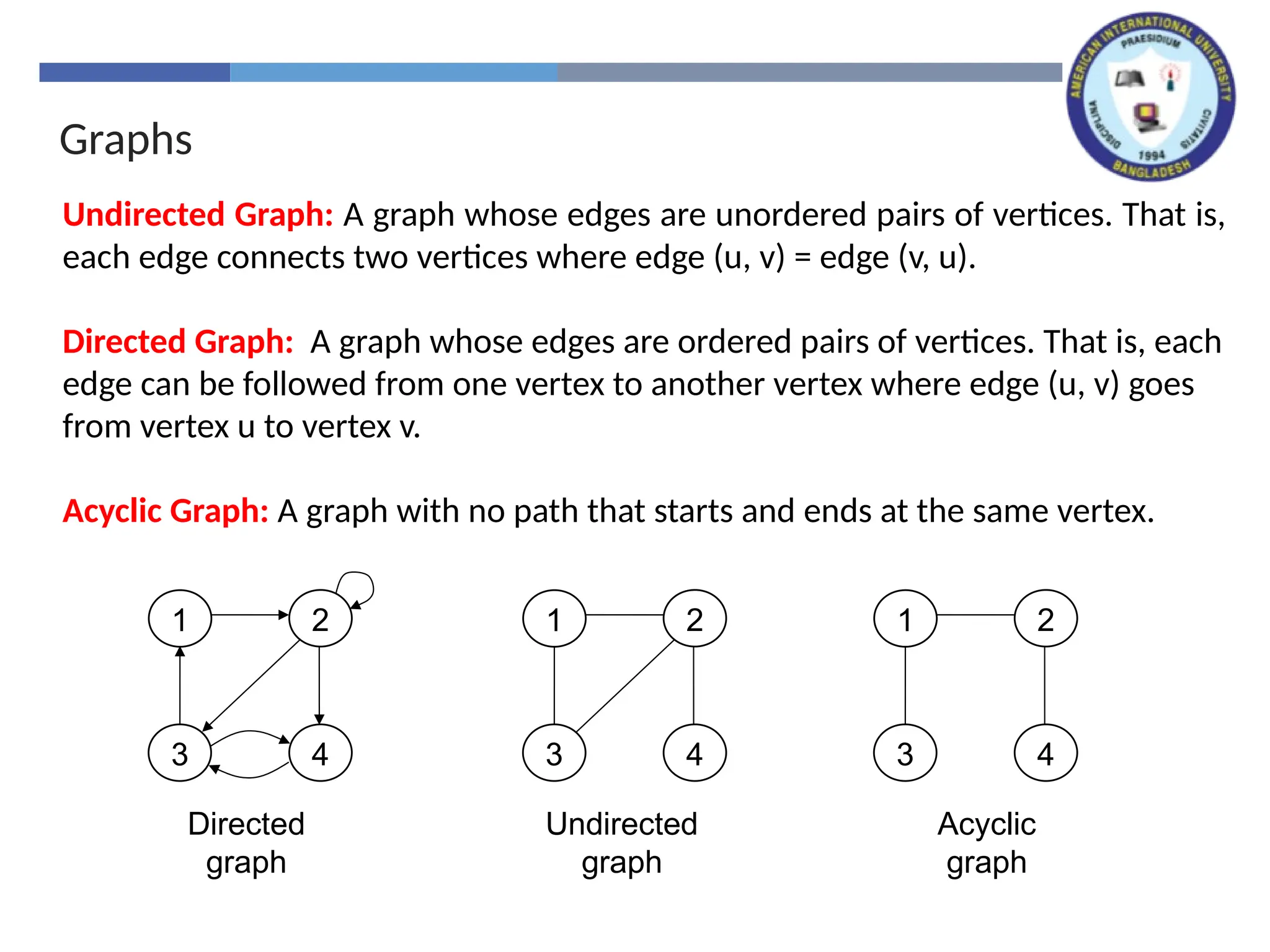
Undirected Graph: A graph whose edges are unordered pairs of vertices. That is,
each edge connects two vertices where edge (u, v) = edge (v, u).
Directed Graph: A graph whose edges are ordered pairs of vertices. That is, each
edge can be followed from one vertex to another vertex where edge (u, v) goes
from vertex u to vertex v.
Acyclic Graph: A graph with no path that starts and ends at the same vertex.
5.
Graph Example
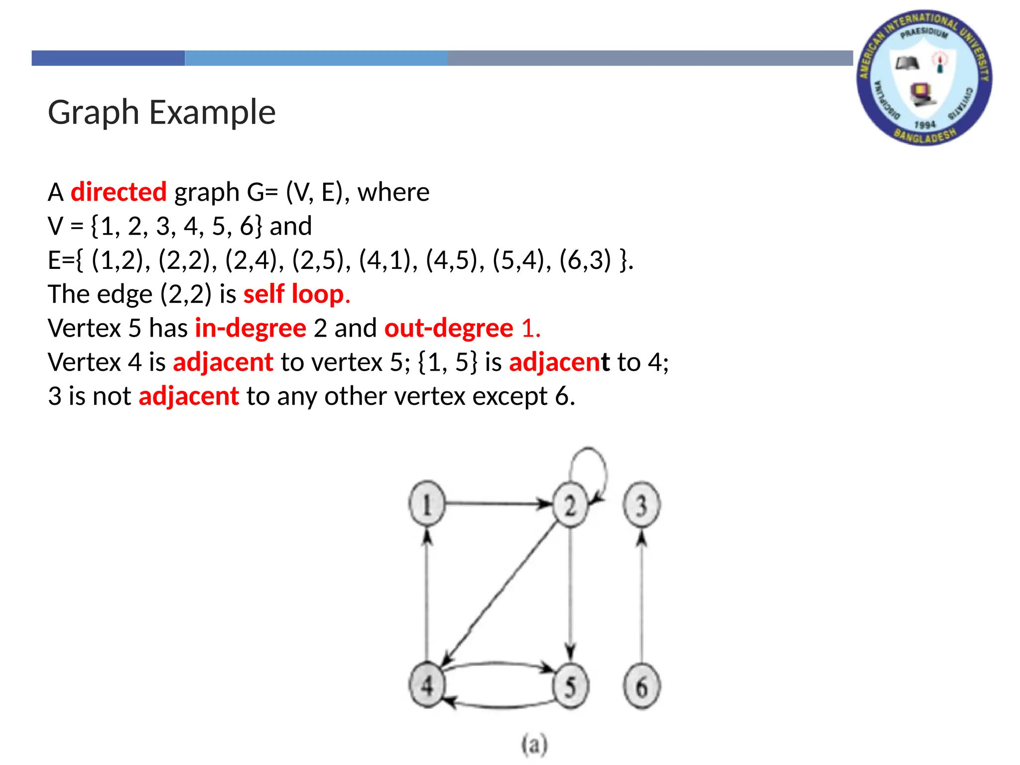
A directedgraph G= (V, E), where
V = {1, 2, 3, 4, 5, 6} and
E={ (1,2), (2,2), (2,4), (2,5), (4,1), (4,5), (5,4), (6,3) }.
The edge (2,2) is self loop.
Vertex 5 has in-degree 2 and out-degree 1.
Vertex 4 is adjacent to vertex 5; {1, 5} is adjacent to 4;
3 is not adjacent to any other vertex except 6.
6.
Graph Example
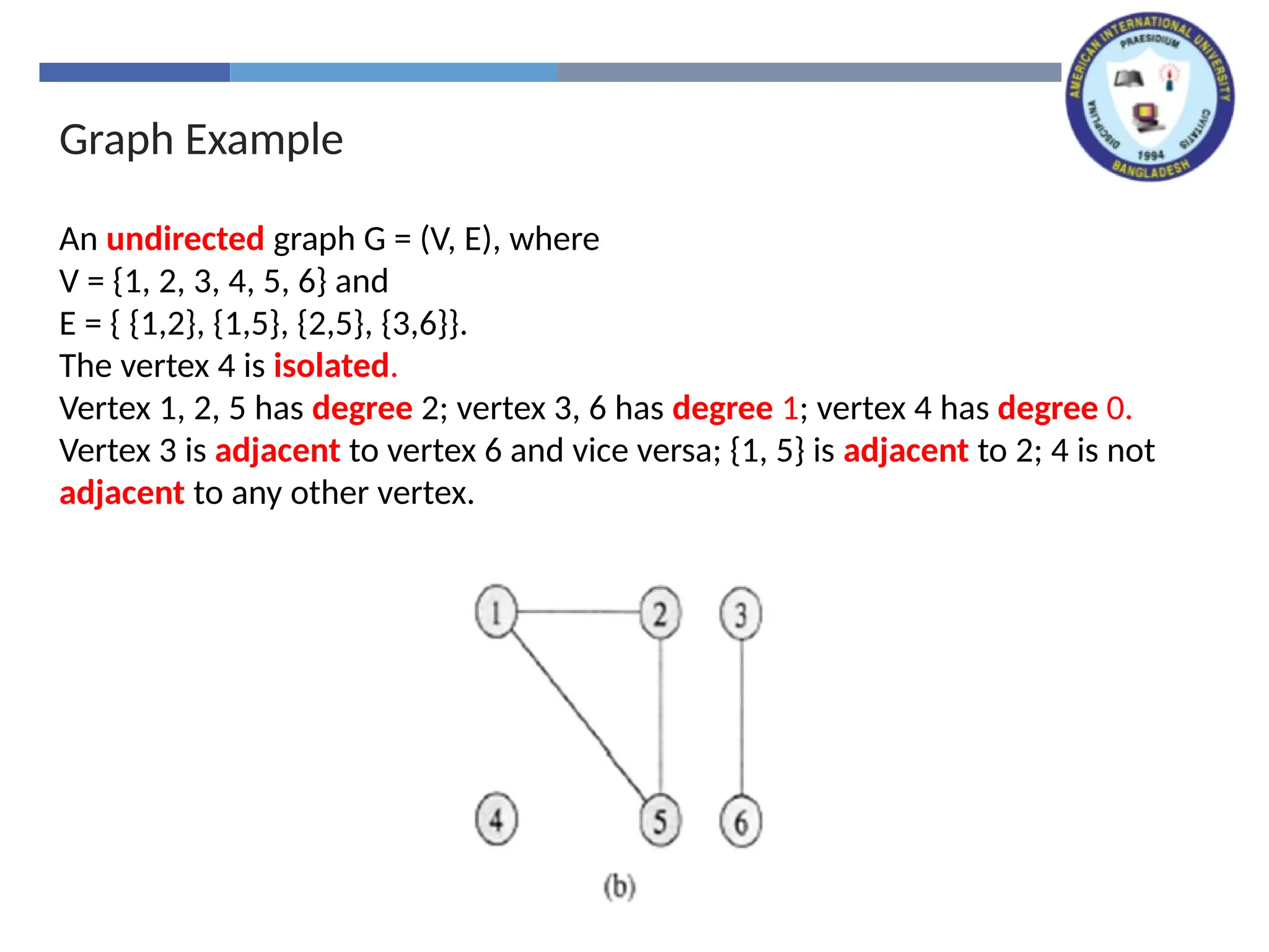
An undirectedgraph G = (V, E), where
V = {1, 2, 3, 4, 5, 6} and
E = { {1,2}, {1,5}, {2,5}, {3,6}}.
The vertex 4 is isolated.
Vertex 1, 2, 5 has degree 2; vertex 3, 6 has degree 1; vertex 4 has degree 0.
Vertex 3 is adjacent to vertex 6 and vice versa; {1, 5} is adjacent to 2; 4 is not
adjacent to any other vertex.
7.
Graph Introduction
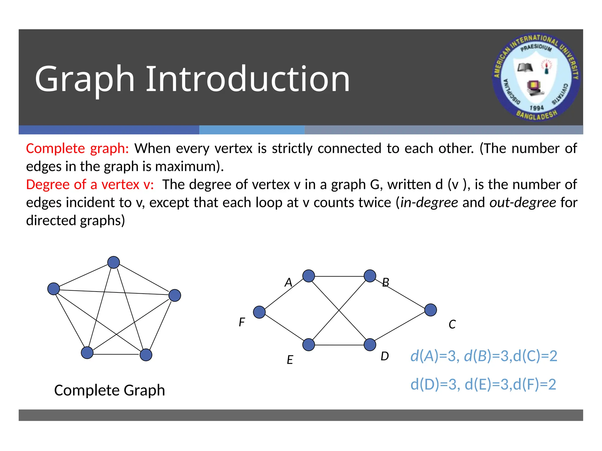
Complete graph:When every vertex is strictly connected to each other. (The number of
edges in the graph is maximum).
Degree of a vertex v: The degree of vertex v in a graph G, written d (v ), is the number of
edges incident to v, except that each loop at v counts twice (in-degree and out-degree for
directed graphs)
Complete Graph
A
C
B
D
F
E d(A)=3, d(B)=3,d(C)=2
d(D)=3, d(E)=3,d(F)=2
8.
Graph Introduction
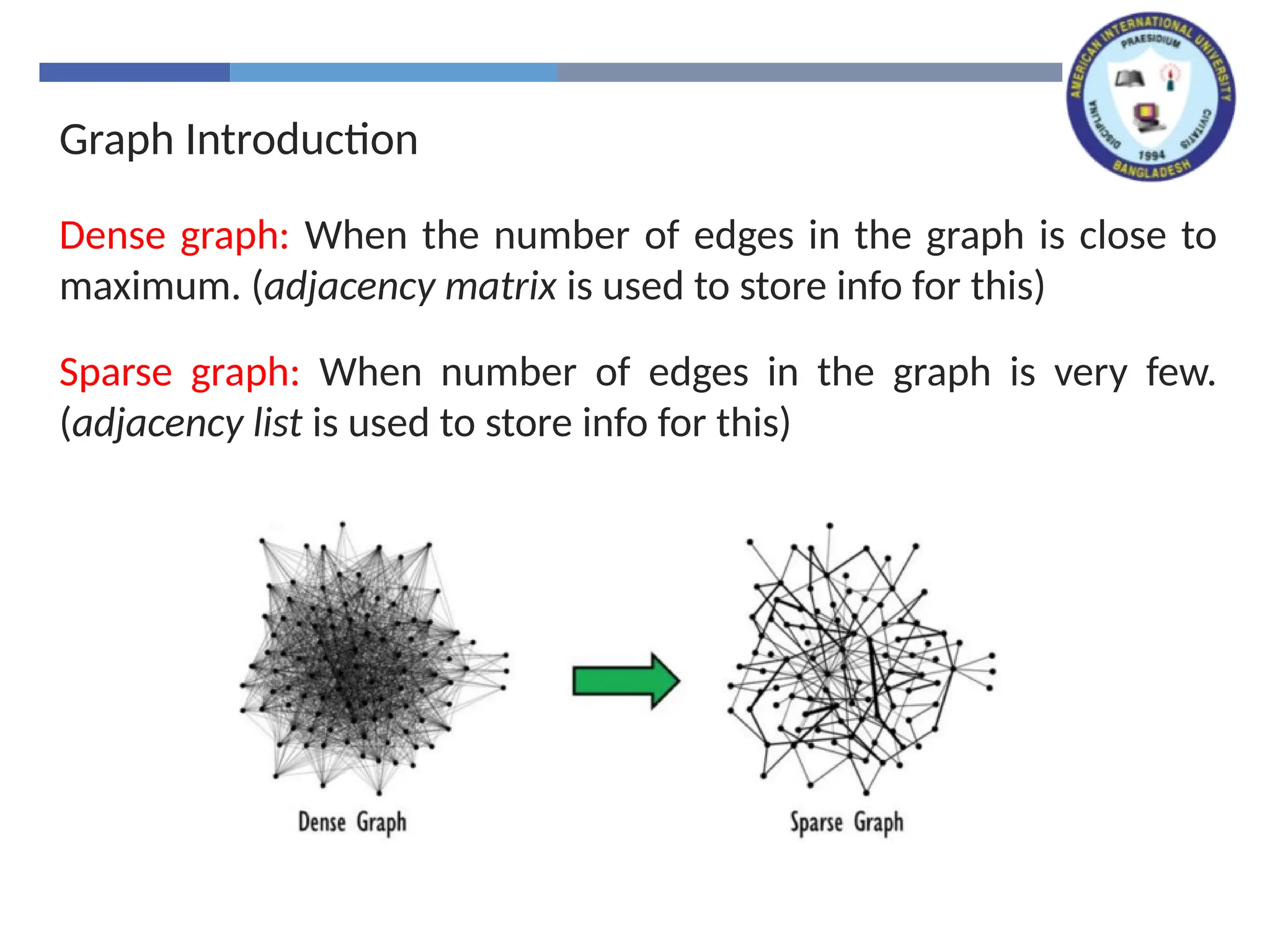
Dense graph:When the number of edges in the graph is close to
maximum. (adjacency matrix is used to store info for this)
Sparse graph: When number of edges in the graph is very few.
(adjacency list is used to store info for this)
9.
Graph Introduction
Weighted graph:associates weights with either the edges or the vertices
DAG: Directed acyclic graphs
Connected: if every vertex of a graph can reach every other vertex, i.e., every
pair of vertices is connected by a path
Strongly connected: every 2 vertices are reachable from each other (in a
digraph)
Connected Component: equivalence classes of vertices under “is reachable
from” relation. Simply put, it is a subgraph in which any two vertices
are connected to each other by paths, and which is connected to no
additional vertices in the supergraph.
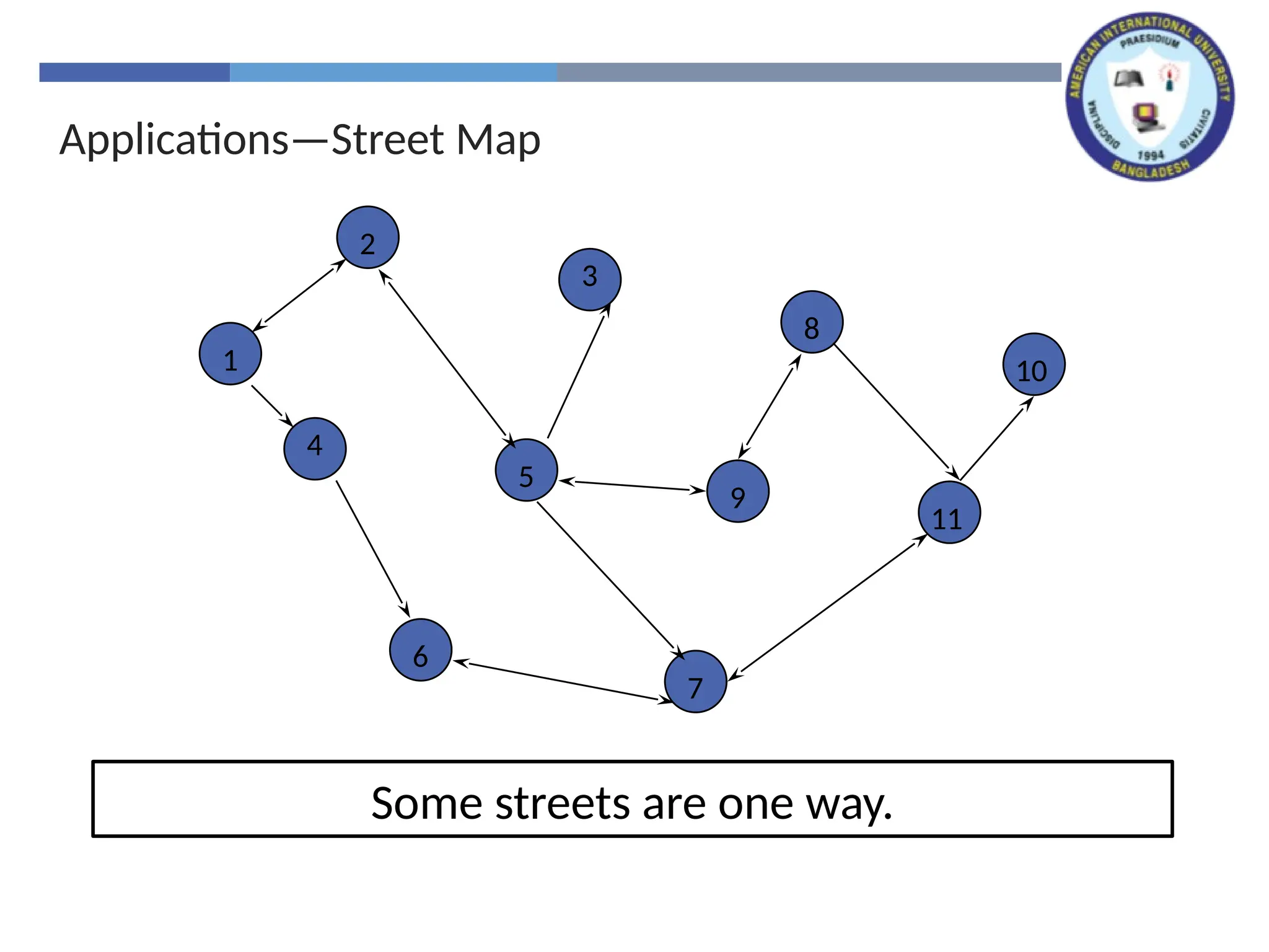
Graph Applications
State-spacesearch in Artificial Intelligence
Geographical information systems, electronic street directory
Logistics and supply chain management
Telecommunications network design
Many more industry applications
The graphic representation of world wide web (www)
Resource allocation graph for processes that are active in the
system.
The graphic representation of a map
Scene graphs: The contents of a visual scene are also managed
by using graph data structure.
Graph Representation
Adjacency matrix:represents a graph as n x n matrix A (here, n is
the number of nodes/ vertices):
A[i, j] = 1 if edge (i, j) E (or weight of edge)
= 0 if edge (i, j) E
Storage requirements: O(n2
)
Using adjacency matrix is more efficient to represent dense
graphs
Especially if store just one bit/edge
Undirected graph: only need half of matrix
16.
Graph Representation
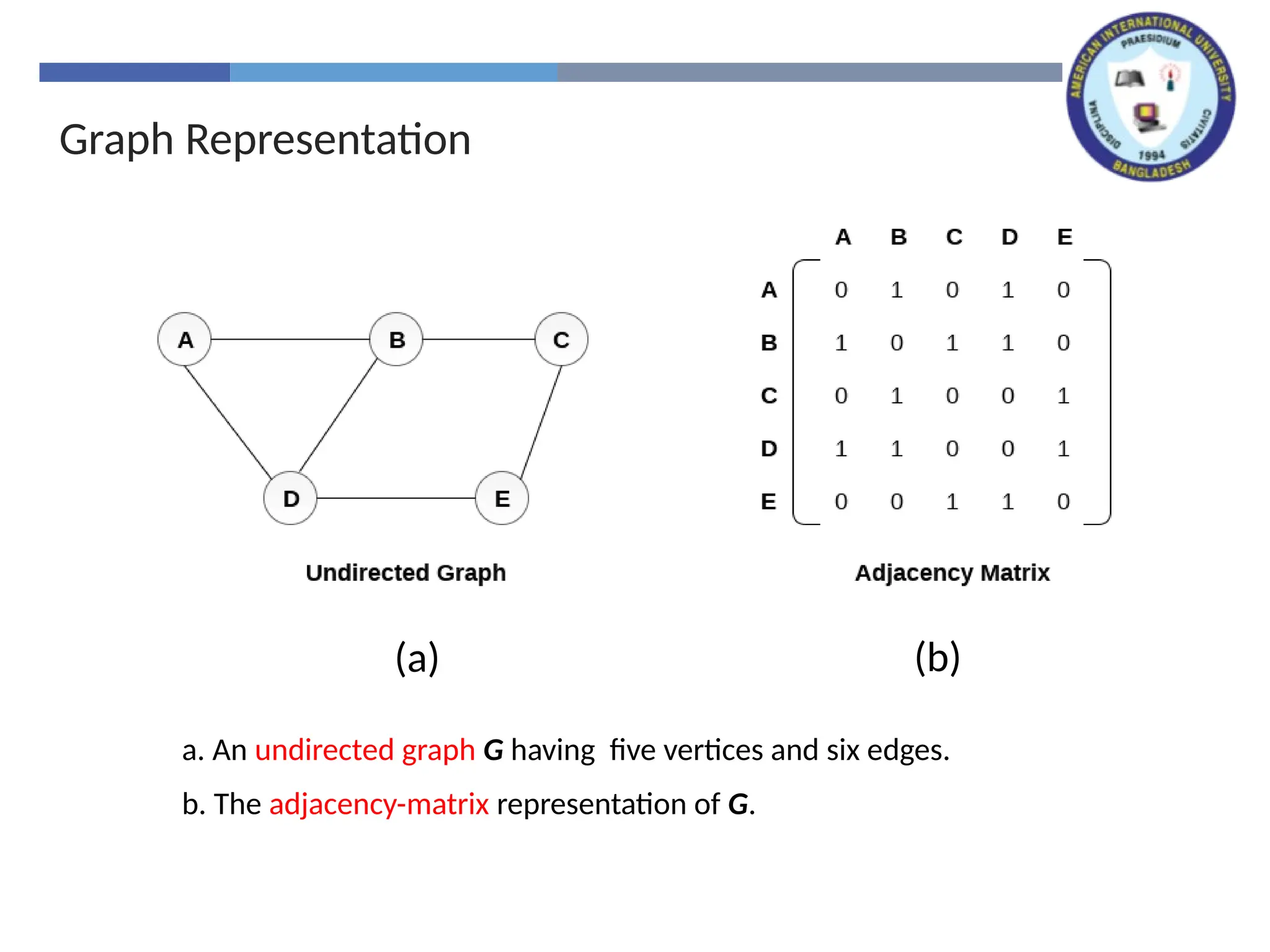
a. Anundirected graph G having five vertices and six edges.
b. The adjacency-matrix representation of G.
(b)
(a)
17.
Graph Representation
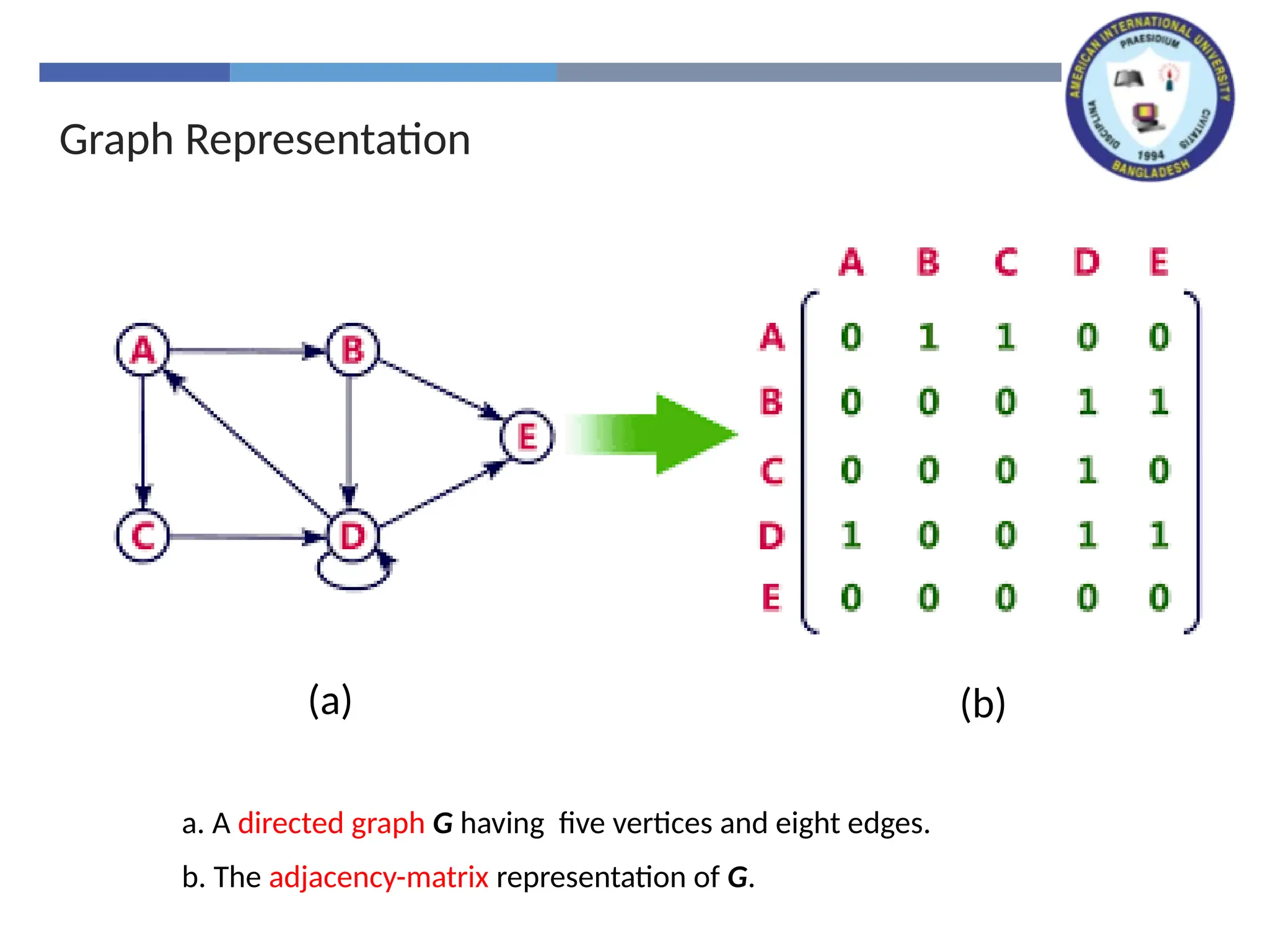
a. Adirected graph G having five vertices and eight edges.
b. The adjacency-matrix representation of G.
(b)
(a)
18.
Graph Representation
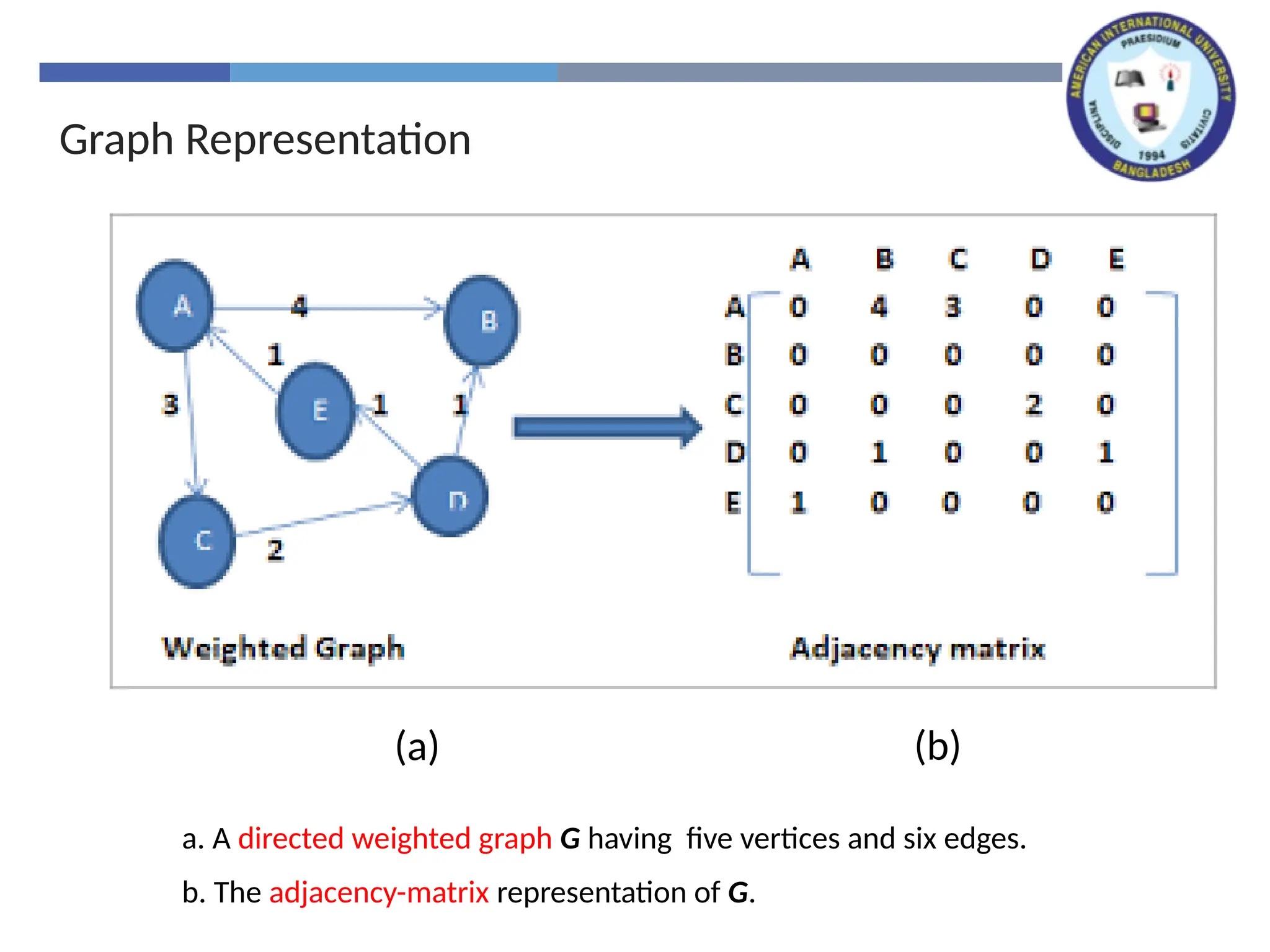
a. Adirected weighted graph G having five vertices and six edges.
b. The adjacency-matrix representation of G.
(b)
(a)
19.
Graph Representation
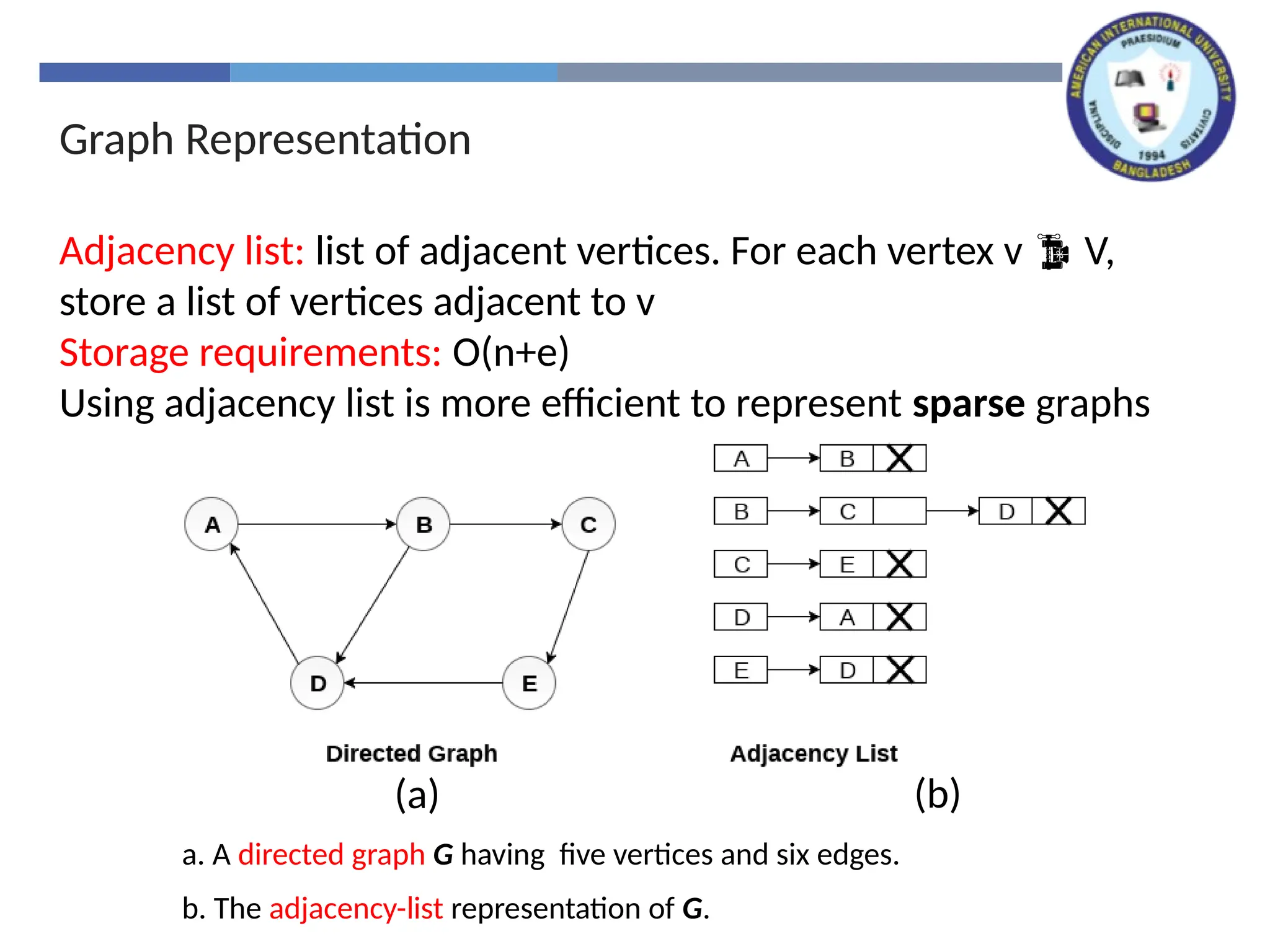
Adjacency list:list of adjacent vertices. For each vertex v V,
store a list of vertices adjacent to v
Storage requirements: O(n+e)
Using adjacency list is more efficient to represent sparse graphs
a. A directed graph G having five vertices and six edges.
b. The adjacency-list representation of G.
(b)
(a)
20.
Graph Representation
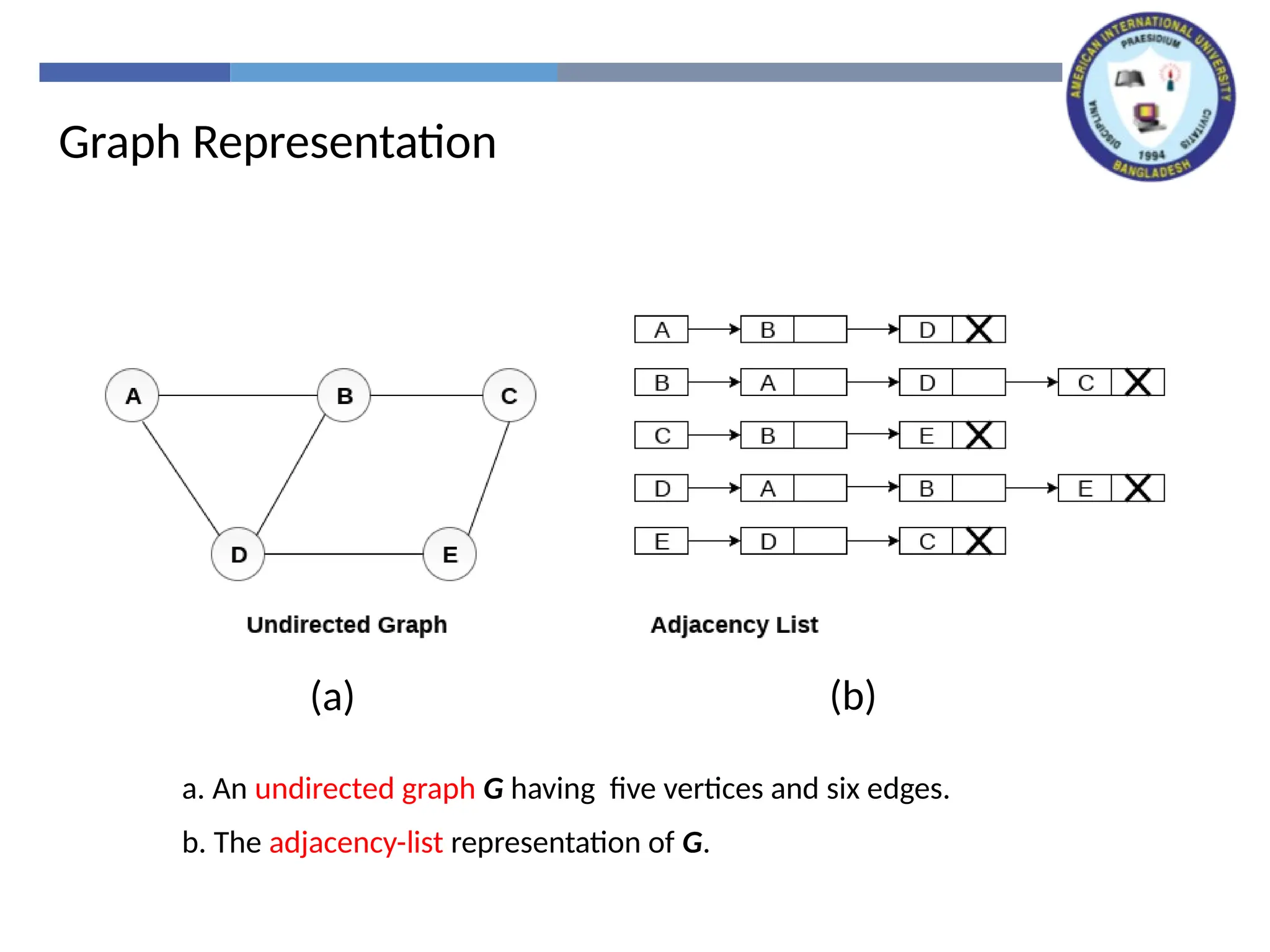
a. Anundirected graph G having five vertices and six edges.
b. The adjacency-list representation of G.
(b)
(a)
21.
Graph Representation
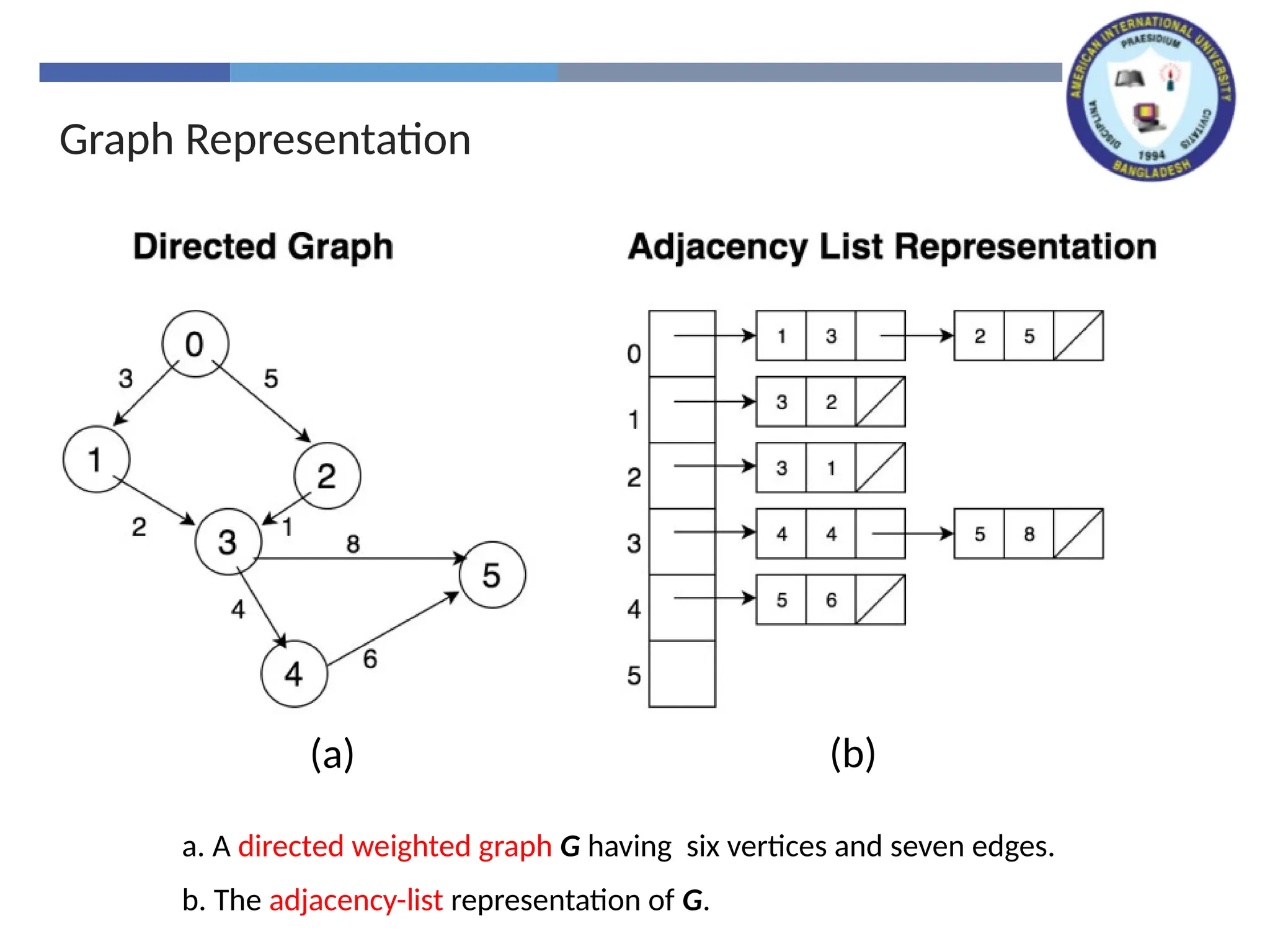
a. Adirected weighted graph G having six vertices and seven edges.
b. The adjacency-list representation of G.
(b)
(a)
22.
Graph Searching
Given:a graph G = (V, E), directed or undirected
Goal: methodically explore every vertex and edge
Ultimately: build a tree on the graph
Pick a vertex as the root
Choose certain edges to produce a tree
Note: might also build a forest if graph is not connected
Breadth-first search
Depth-first search
Other variants: best-first, iterated deepening search, etc.
23.
Depth-First Search (DFS)
Explore “deeper” in the graph whenever possible
Edges are explored out of the most recently discovered vertex v that still has
unexplored edges (LIFO)
When all of v’s edges have been explored, backtrack to the vertex from which
v was discovered
computes 2 timestamps: d[ ] (discovered) and f[ ] (finished)
builds one or more depth-first tree(s) (depth-first forest)
Algorithm colors each vertex
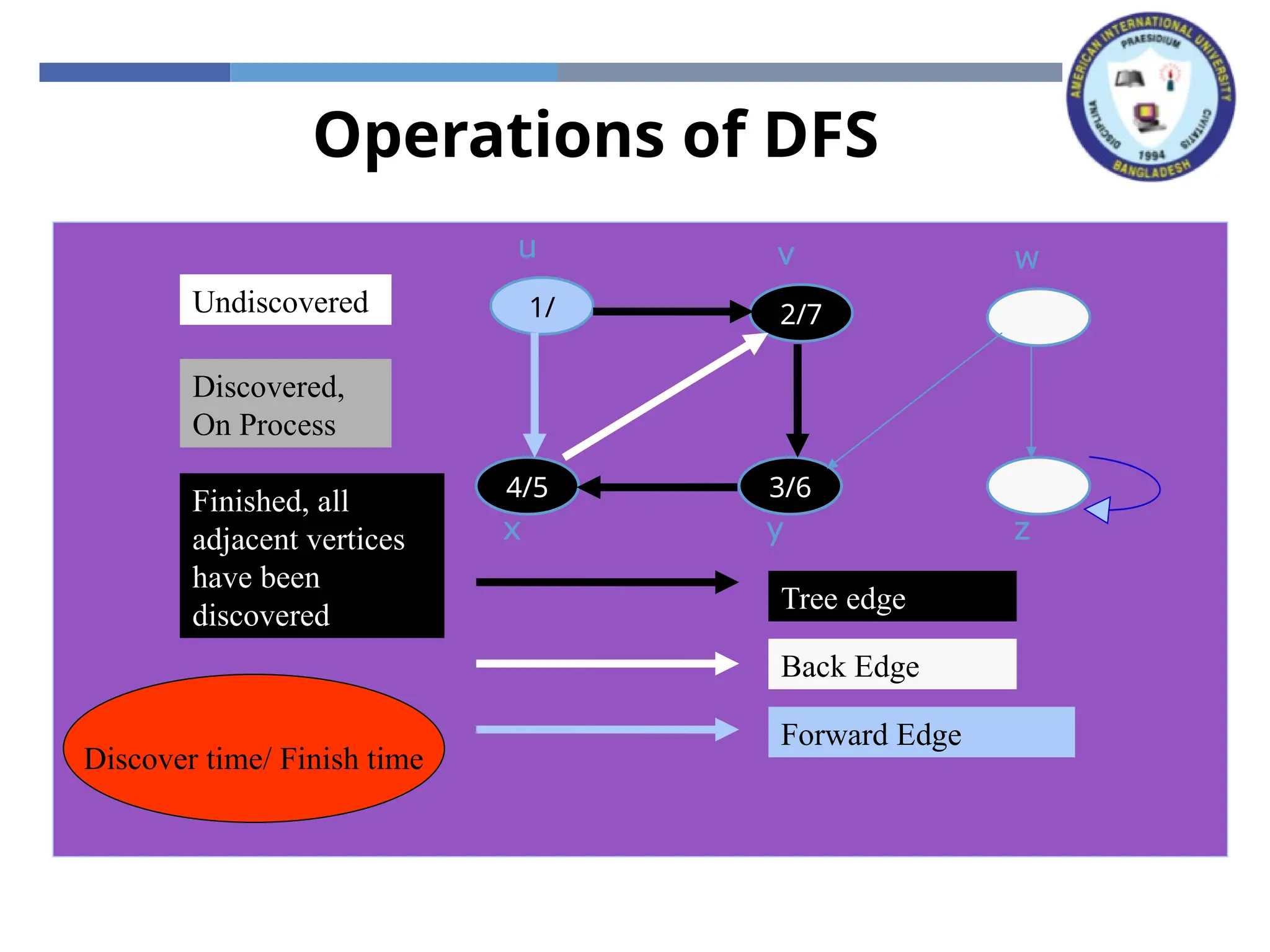
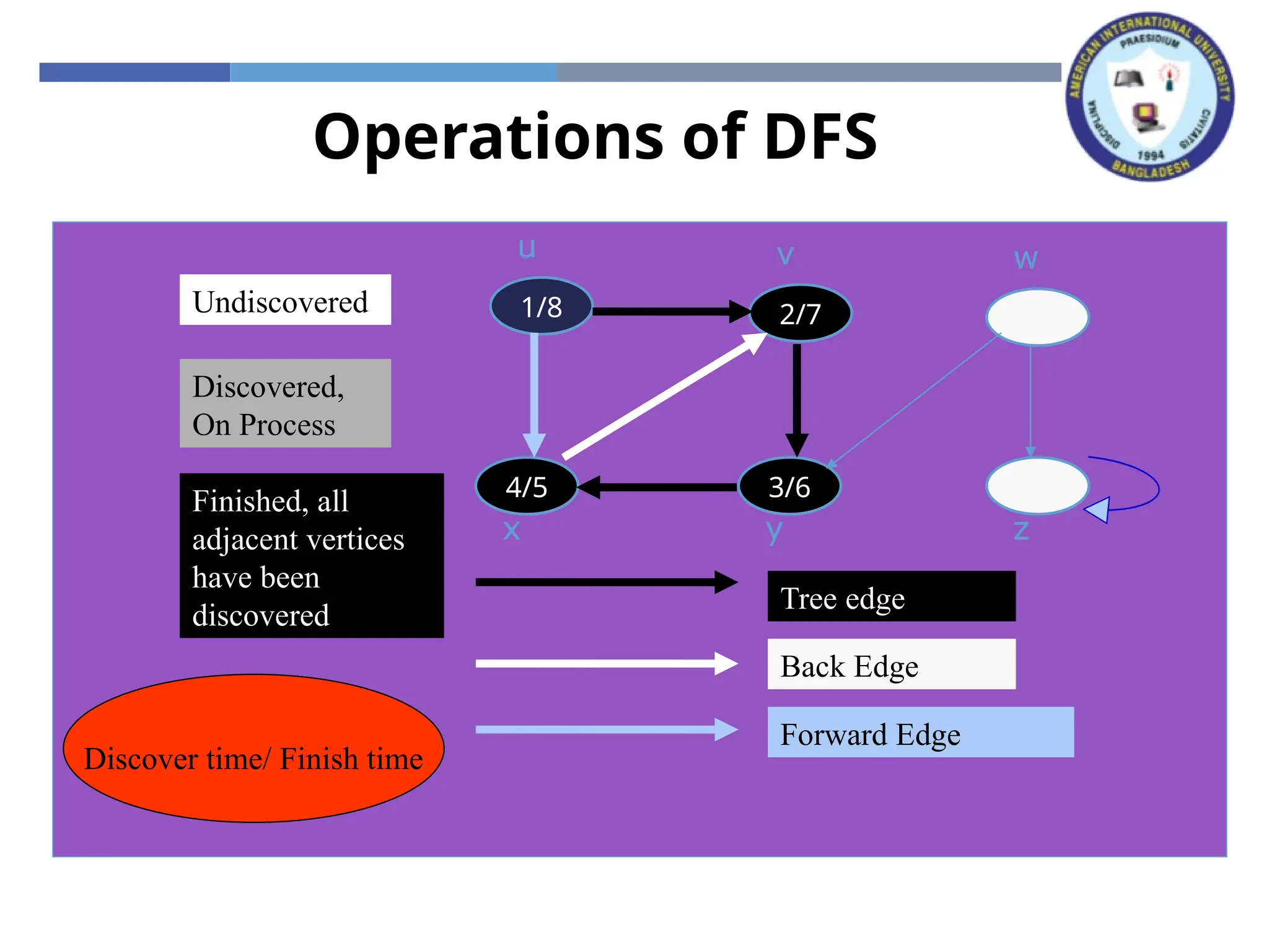
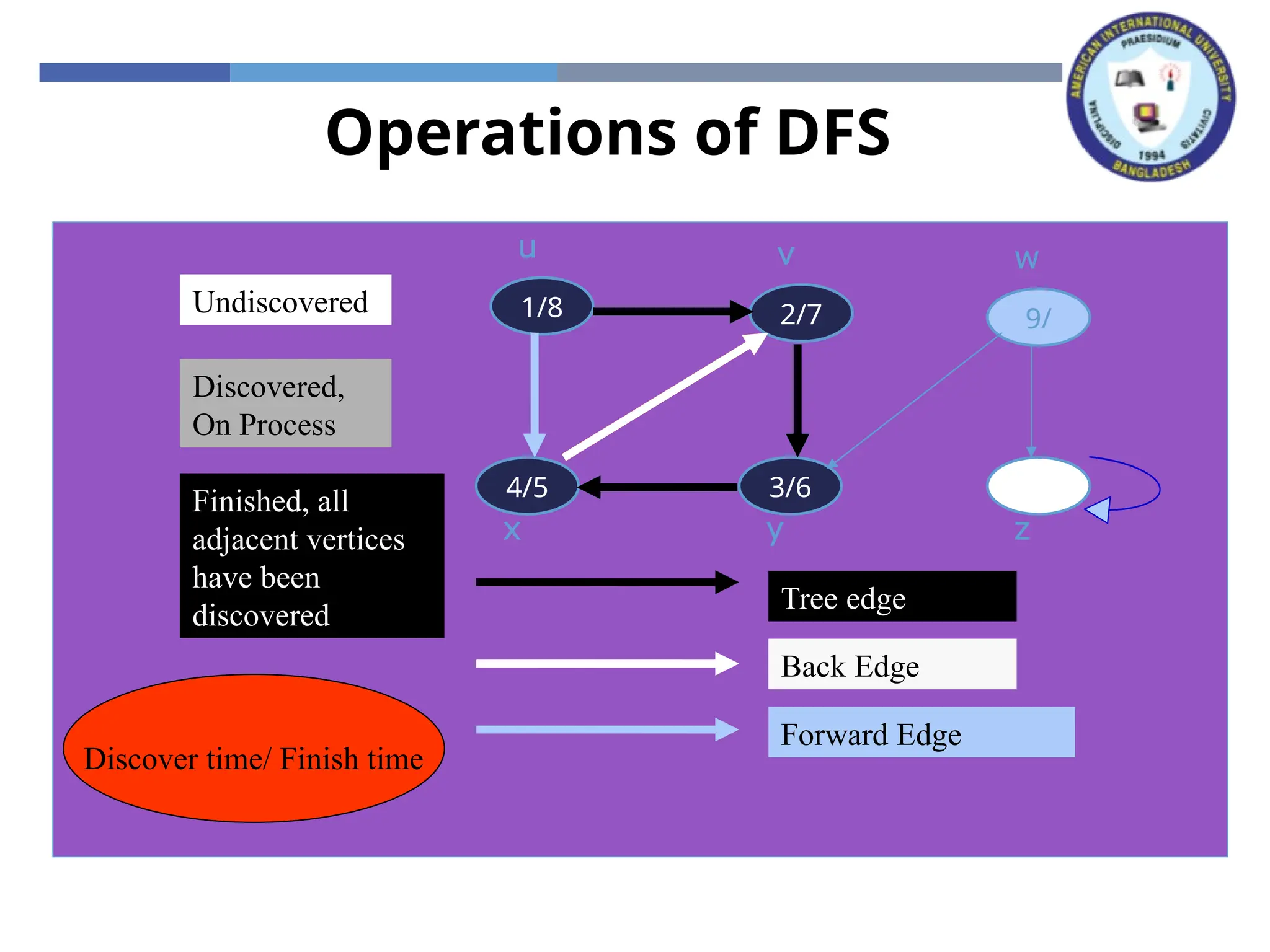
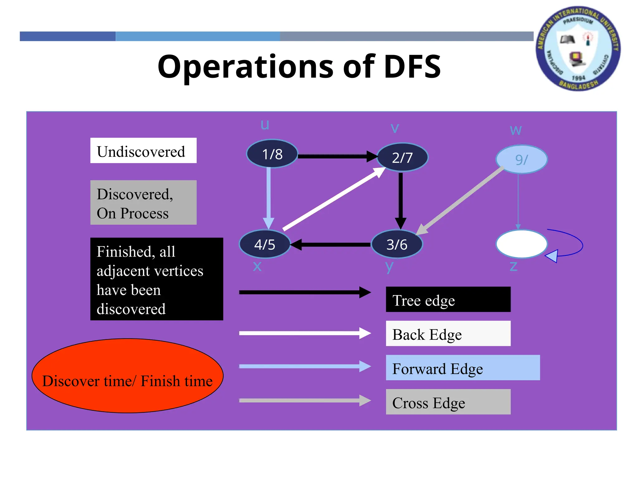
WHITE: undiscovered
GRAY: discovered, in process
BLACK: finished, all adjacent vertices have been discovered
24.
Depth-First Search: TheCode
DFS(G)
{
for each vertex u V
color[u] = WHITE;
time = 0;
for each vertex u V
if (color[u] == WHITE)
DFS_Visit(u);
}
DFS_Visit(u)
{
color[u] = GREY;
time = time+1;
d[u] = time; // compute d[]
for each v adjacent to u
if (color[v] == WHITE)
p[v]= u // build tree
DFS_Visit(v);
color[u] = BLACK;
time = time+1;
f[u] = time; // compute f[]
}
25.
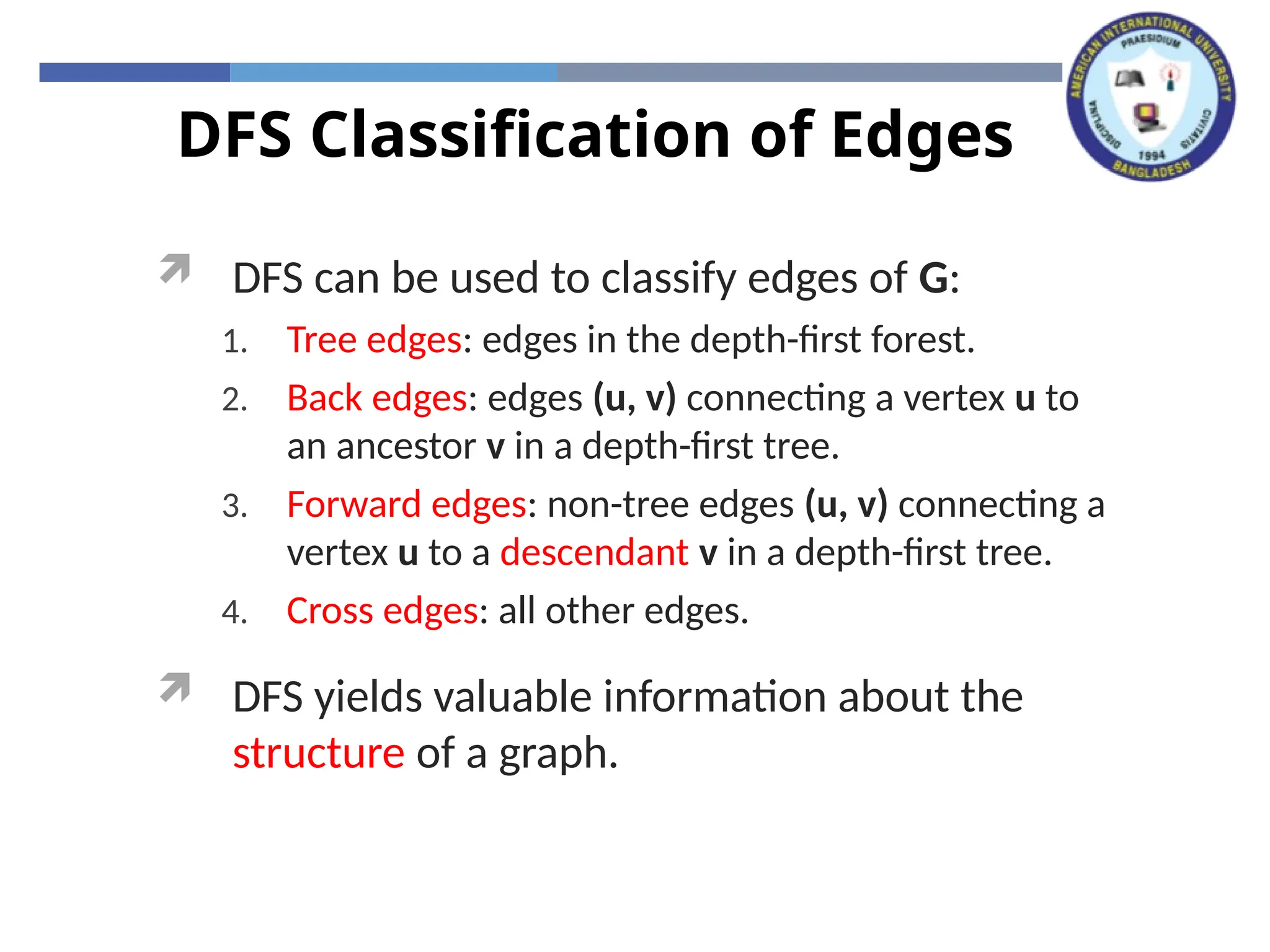
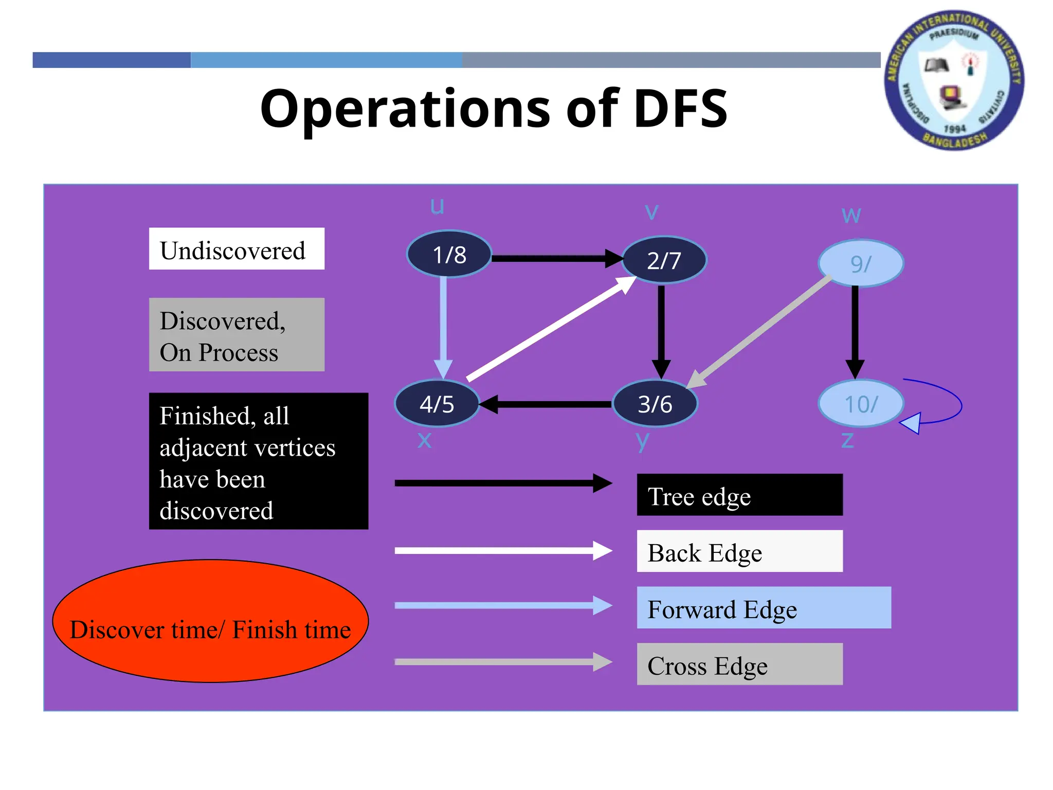
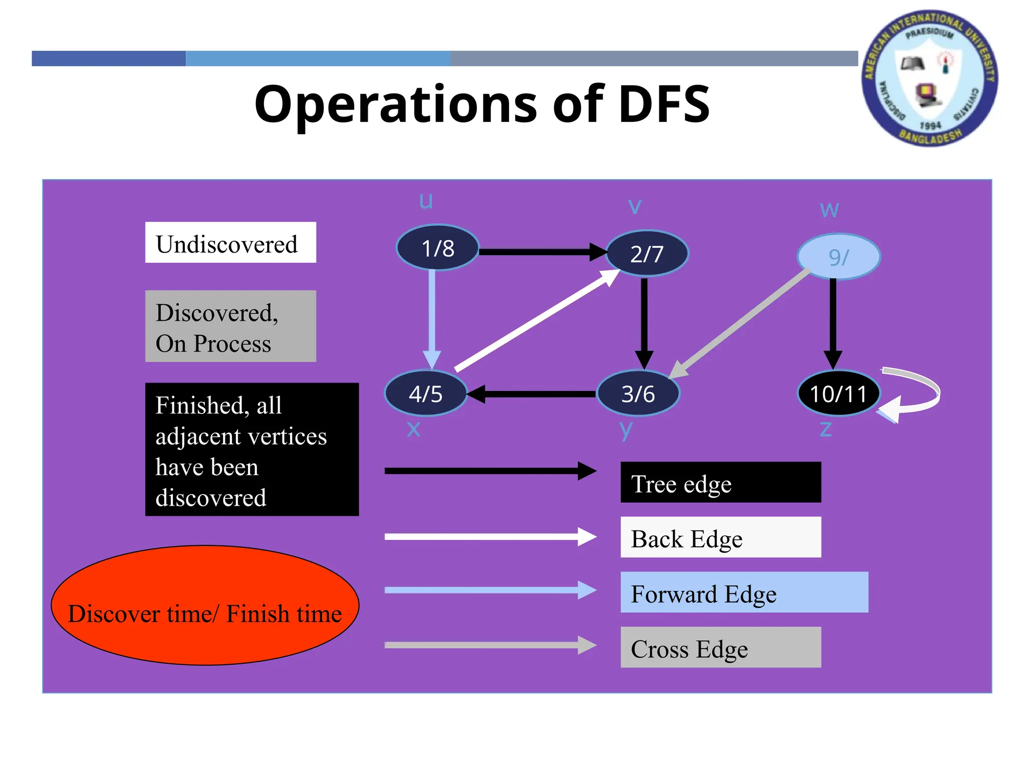
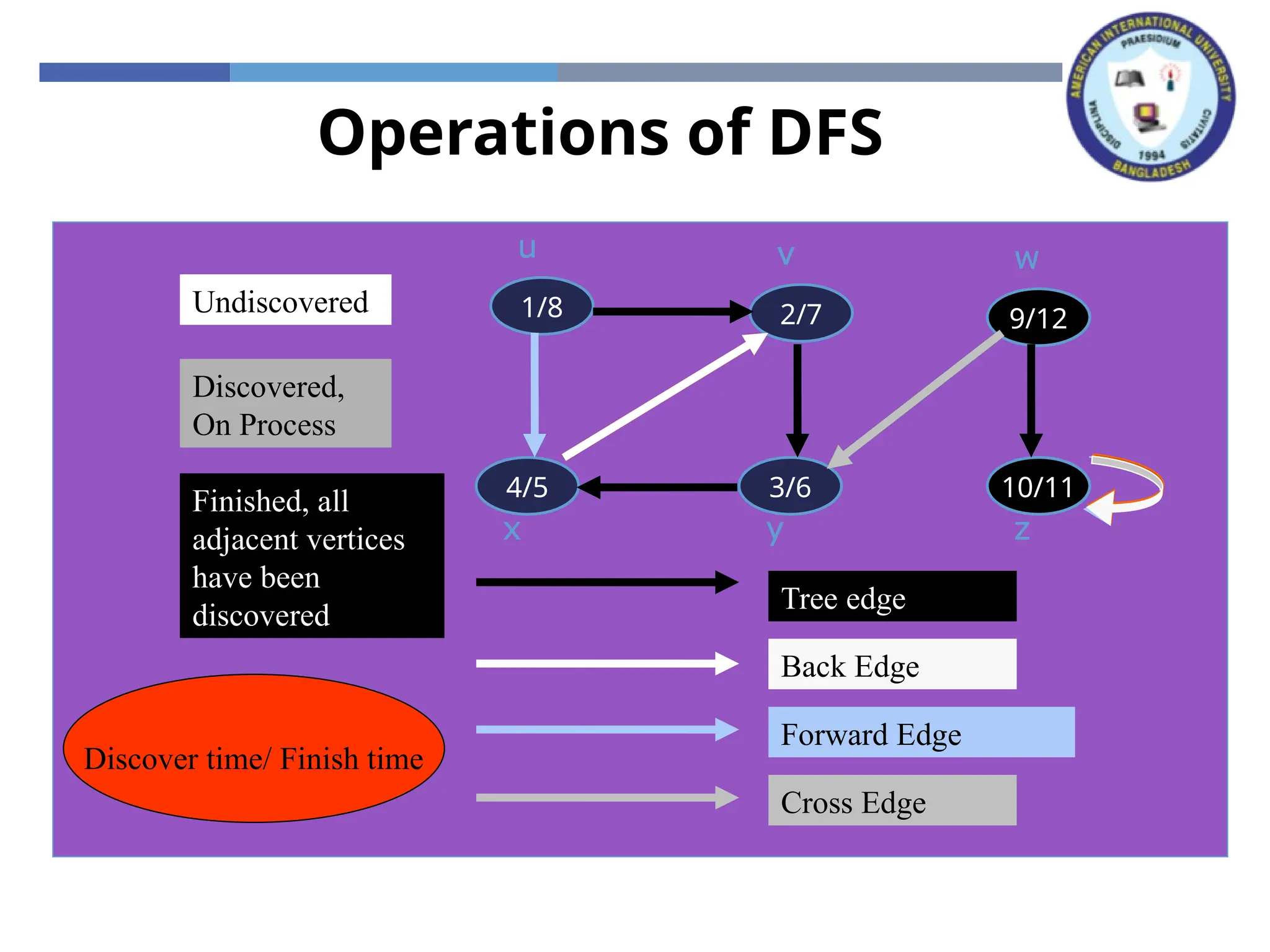
DFS Classification ofEdges
DFS can be used to classify edges of G:
1. Tree edges: edges in the depth-first forest.
2. Back edges: edges (u, v) connecting a vertex u to
an ancestor v in a depth-first tree.
3. Forward edges: non-tree edges (u, v) connecting a
vertex u to a descendant v in a depth-first tree.
4. Cross edges: all other edges.
DFS yields valuable information about the
structure of a graph.
26.
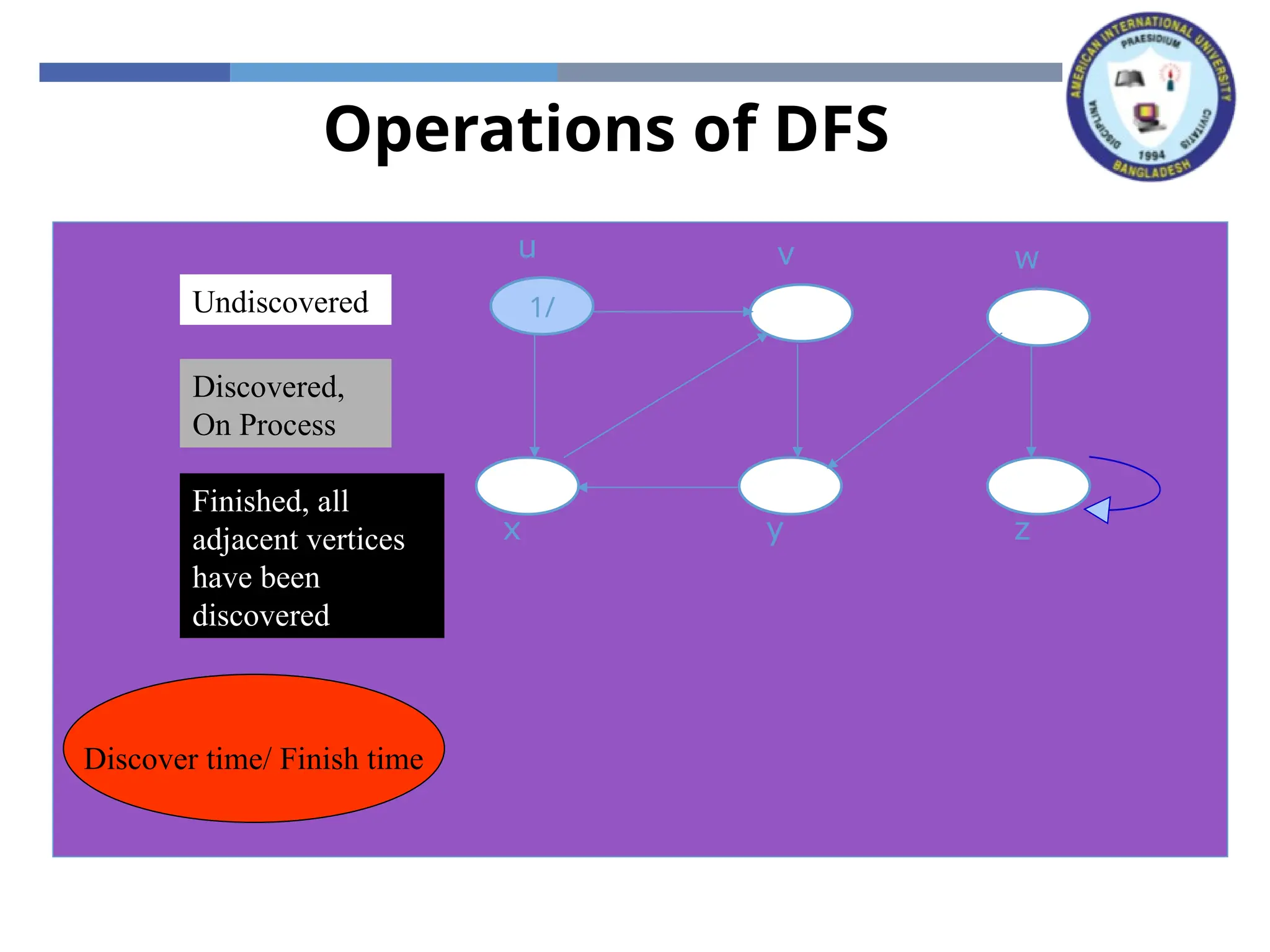
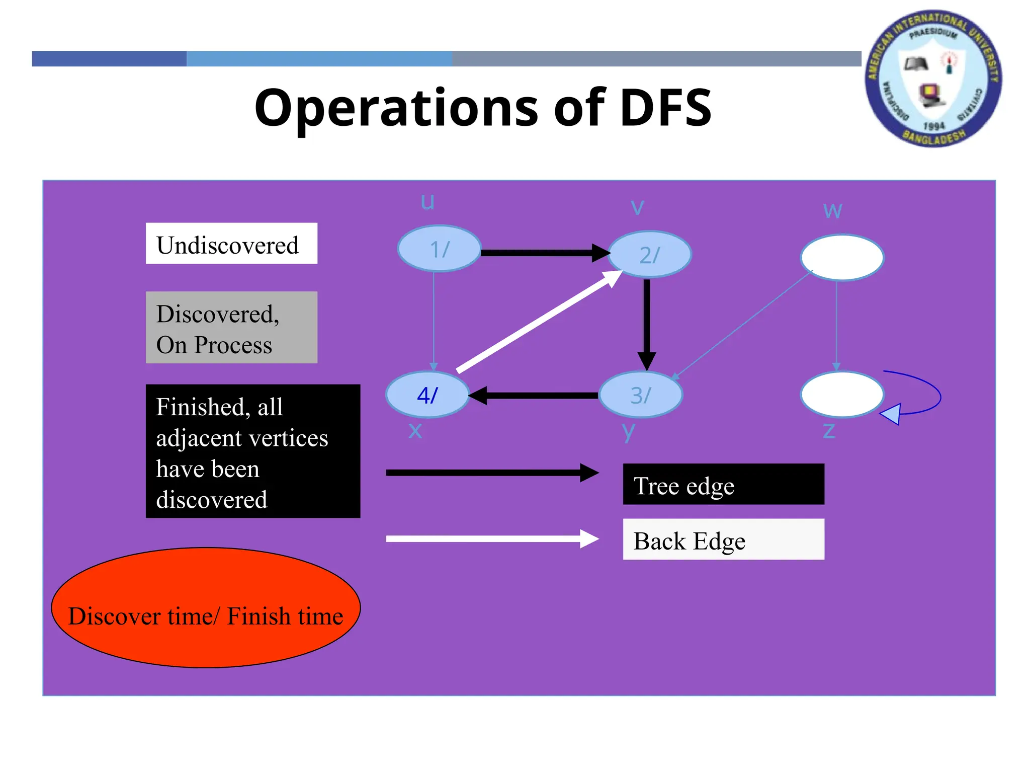
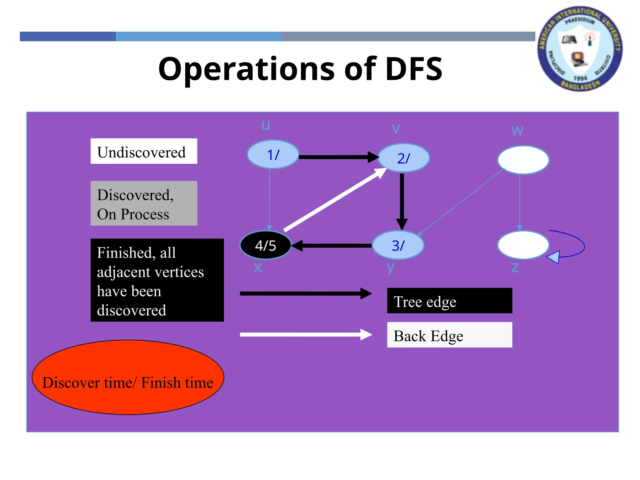
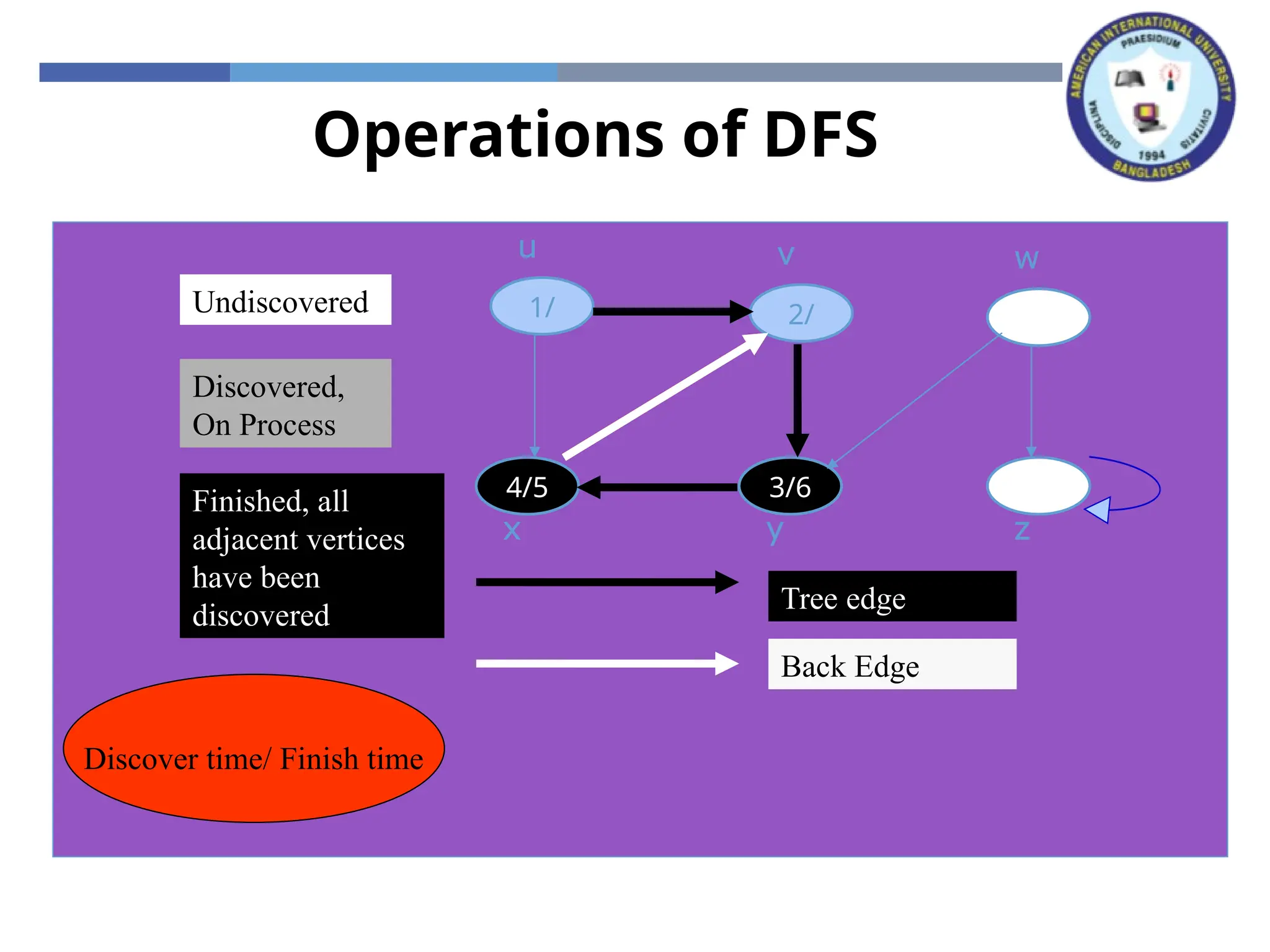
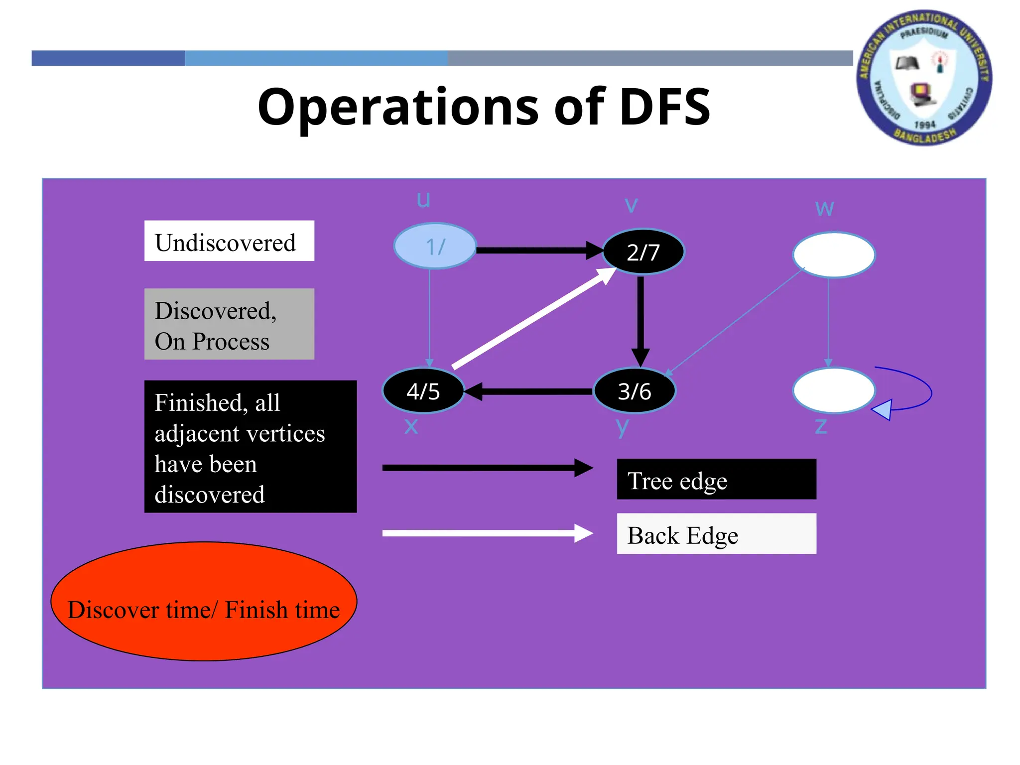
Operations of DFS
xz
y
w
v
u
Undiscovered
Discovered,
On Process
Finished, all
adjacent vertices
have been
discovered
Discover time/ Finish time
27.
Operations of DFS
xz
y
w
v
u
x z
y
w
v
1/
u
Undiscovered
Discovered,
On Process
Finished, all
adjacent vertices
have been
discovered
Discover time/ Finish time
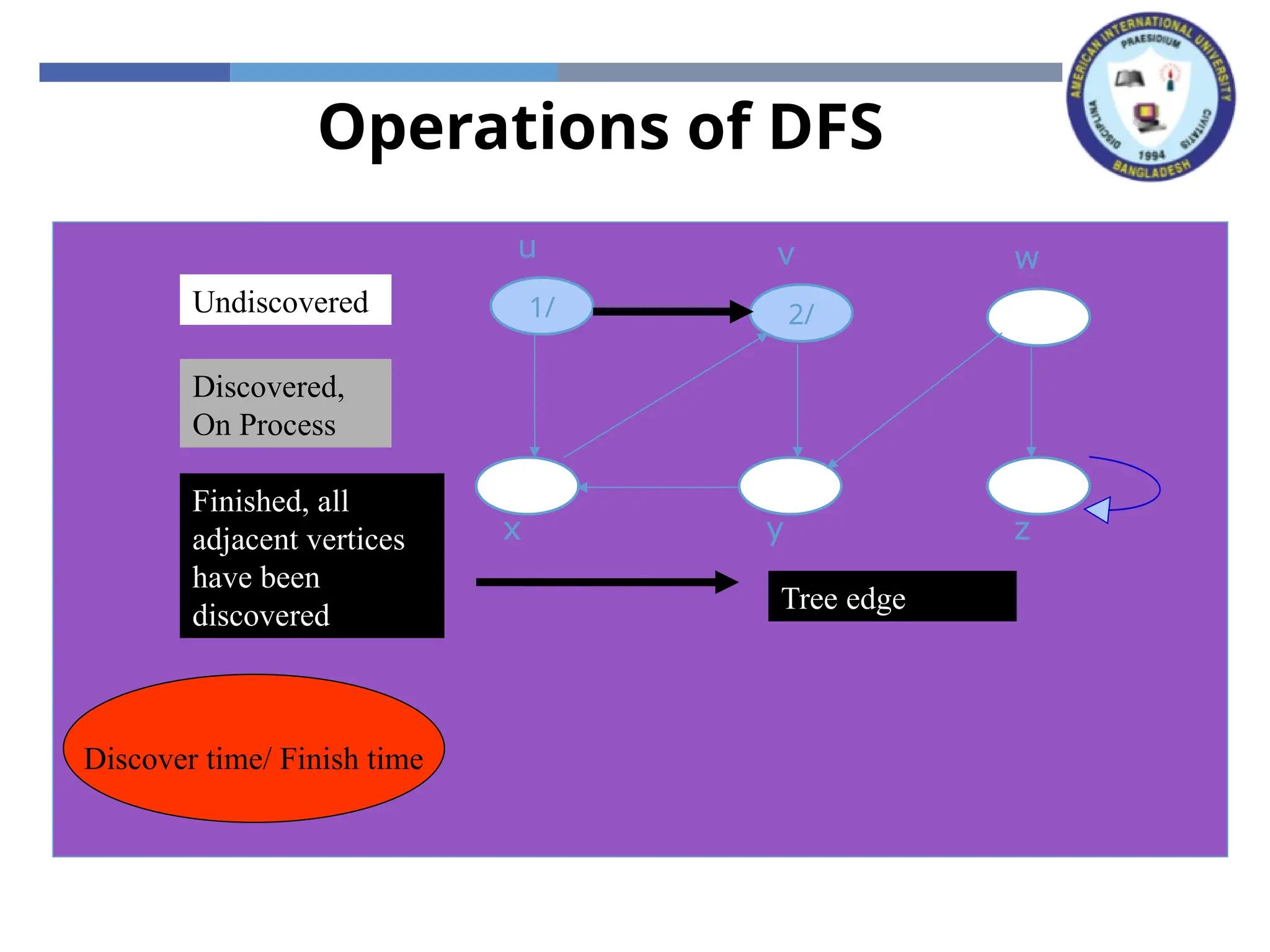
28.
Operations of DFS
xz
y
w
v
u
x z
y
w
v
1/
u
x z
y
w
2/
v
1/
u
Tree edge
Undiscovered
Discovered,
On Process
Finished, all
adjacent vertices
have been
discovered
Discover time/ Finish time
29.
Operations of DFS
xz
y
w
v
u
x z
y
w
v
1/
u
x z
y
w
2/
v
1/
u
Tree edge
x z
3/
y
w
2/
v
1/
u
Undiscovered
Discovered,
On Process
Finished, all
adjacent vertices
have been
discovered
Discover time/ Finish time
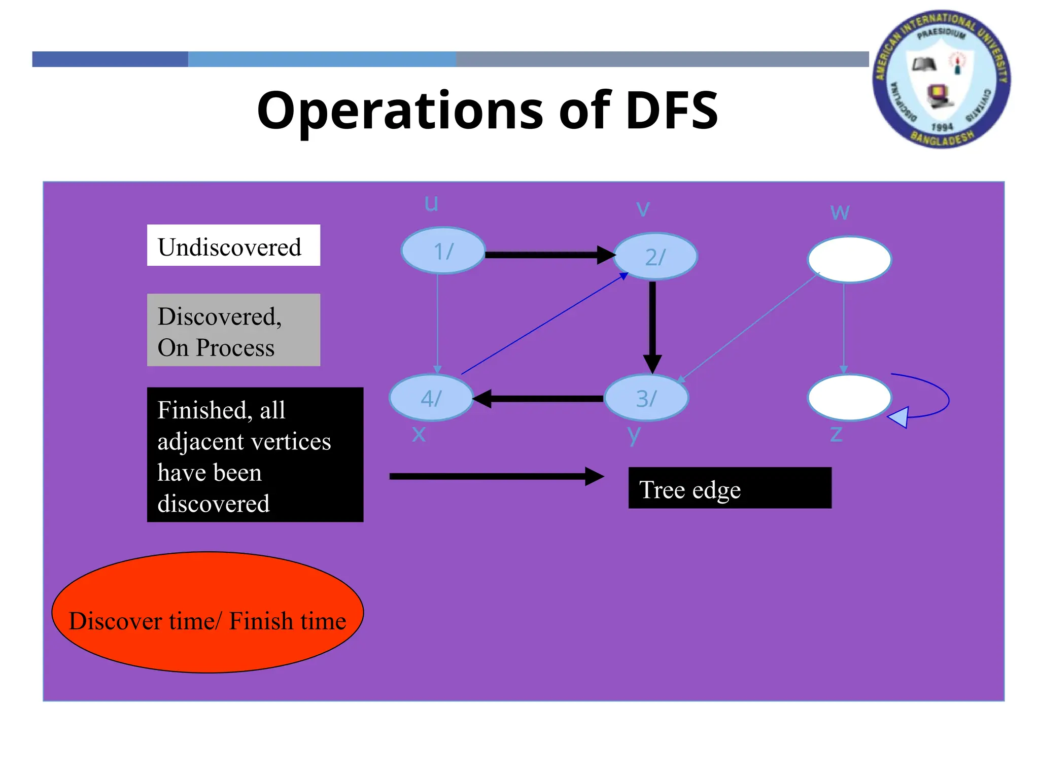
30.
Operations of DFS
xz
y
w
v
u
x z
y
w
v
1/
u
x z
y
w
2/
v
1/
u
Tree edge
x z
3/
y
w
2/
v
1/
u
4/
x z
3/
y
w
2/
v
1/
u
Undiscovered
Discovered,
On Process
Finished, all
adjacent vertices
have been
discovered
Discover time/ Finish time
31.
Operations of DFS
xz
y
w
v
u
x z
y
w
v
1/
u
x z
y
w
2/
v
1/
u
Tree edge
x z
3/
y
w
2/
v
1/
u
4/
x z
3/
y
w
2/
v
1/
u
4/
x z
3/
y
w
2/
v
1/
u
Back Edge
Undiscovered
Discovered,
On Process
Finished, all
adjacent vertices
have been
discovered
Discover time/ Finish time
32.
Operations of DFS
xz
y
w
v
u
x z
y
w
v
1/
u
x z
y
w
2/
v
1/
u
Tree edge
x z
3/
y
w
2/
v
1/
u
4/
x z
3/
y
w
2/
v
1/
u
4/
x z
3/
y
w
2/
v
1/
u
Back Edge
4/5
x z
3/
y
w
2/
v
1/
u
Undiscovered
Discovered,
On Process
Finished, all
adjacent vertices
have been
discovered
Discover time/ Finish time
33.
Operations of DFS
xz
y
w
v
u
x z
y
w
v
1/
u
x z
y
w
2/
v
1/
u
Tree edge
x z
3/
y
w
2/
v
1/
u
4/
x z
3/
y
w
2/
v
1/
u
4/
x z
3/
y
w
2/
v
1/
u
Back Edge
4/5
x z
3/
y
w
2/
v
1/
u
4/5
x z
3/6
y
w
2/
v
1/
u
Undiscovered
Discovered,
On Process
Finished, all
adjacent vertices
have been
discovered
Discover time/ Finish time
34.
Operations of DFS
xz
y
w
v
u
x z
y
w
v
1/
u
x z
y
w
2/
v
1/
u
Tree edge
x z
3/
y
w
2/
v
1/
u
4/
x z
3/
y
w
2/
v
1/
u
4/
x z
3/
y
w
2/
v
1/
u
Back Edge
4/5
x z
3/
y
w
2/
v
1/
u
4/5
x z
3/6
y
w
2/
v
1/
u
4/5
x z
3/6
y
w
2/7
v
1/
u
Undiscovered
Discovered,
On Process
Finished, all
adjacent vertices
have been
discovered
Discover time/ Finish time
35.
Operations of DFS
xz
y
w
v
u
x z
y
w
v
1/
u
x z
y
w
2/
v
1/
u
Tree edge
x z
3/
y
w
2/
v
1/
u
4/
x z
3/
y
w
2/
v
1/
u
4/
x z
3/
y
w
2/
v
1/
u
Back Edge
4/5
x z
3/
y
w
2/
v
1/
u
4/5
x z
3/6
y
w
2/
v
1/
u
4/5
x z
3/6
y
w
2/7
v
1/
u
4/5
x z
3/6
y
w
2/7
v
1/8
u
4/5
x z
3/6
y
w
2/7
v
1/
u
Forward Edge
Undiscovered
Discovered,
On Process
Finished, all
adjacent vertices
have been
discovered
Discover time/ Finish time
36.
Operations of DFS
xz
y
w
v
u
x z
y
w
v
1/
u
x z
y
w
2/
v
1/
u
Tree edge
x z
3/
y
w
2/
v
1/
u
4/
x z
3/
y
w
2/
v
1/
u
4/
x z
3/
y
w
2/
v
1/
u
Back Edge
4/5
x z
3/
y
w
2/
v
1/
u
4/5
x z
3/6
y
w
2/
v
1/
u
4/5
x z
3/6
y
w
2/7
v
1/
u
4/5
x z
3/6
y
w
2/7
v
1/8
u
Undiscovered
Discovered,
On Process
Finished, all
adjacent vertices
have been
discovered
Discover time/ Finish time
4/5
x z
3/6
y
w
2/7
v
1/8
u
Forward Edge
37.
Operations of DFS
xz
y
w
v
u
x z
y
w
v
1/
u
x z
y
w
2/
v
1/
u
Tree edge
x z
3/
y
w
2/
v
1/
u
4/
x z
3/
y
w
2/
v
1/
u
4/
x z
3/
y
w
2/
v
1/
u
Back Edge
4/5
x z
3/
y
w
2/
v
1/
u
4/5
x z
3/6
y
w
2/
v
1/
u
4/5
x z
3/6
y
w
2/7
v
1/
u
4/5
x z
3/6
y
w
2/7
v
1/8
u
4/5
x z
3/6
y
w
2/7
v
1/8
u
Forward Edge
4/5
x z
3/6
y
9/
w
2/7
v
1/8
u
Undiscovered
Discovered,
On Process
Finished, all
adjacent vertices
have been
discovered
Discover time/ Finish time
38.
Operations of DFS
xz
y
w
v
u
x z
y
w
v
1/
u
x z
y
w
2/
v
1/
u
Tree edge
x z
3/
y
w
2/
v
1/
u
4/
x z
3/
y
w
2/
v
1/
u
4/
x z
3/
y
w
2/
v
1/
u
Back Edge
4/5
x z
3/
y
w
2/
v
1/
u
4/5
x z
3/6
y
w
2/
v
1/
u
4/5
x z
3/6
y
w
2/7
v
1/
u
4/5
x z
3/6
y
w
2/7
v
1/8
u
4/5
x z
3/6
y
w
2/7
v
1/8
u
Forward Edge
4/5
x z
3/6
y
9/
w
2/7
v
1/8
u
4/5
x z
3/6
y
9/
w
2/7
v
1/8
u
Cross Edge
Undiscovered
Discovered,
On Process
Finished, all
adjacent vertices
have been
discovered
Discover time/ Finish time
39.
Operations of DFS
xz
y
w
v
u
x z
y
w
v
1/
u
x z
y
w
2/
v
1/
u
Tree edge
x z
3/
y
w
2/
v
1/
u
4/
x z
3/
y
w
2/
v
1/
u
4/
x z
3/
y
w
2/
v
1/
u
Back Edge
4/5
x z
3/
y
w
2/
v
1/
u
4/5
x z
3/6
y
w
2/
v
1/
u
4/5
x z
3/6
y
w
2/7
v
1/
u
4/5
x z
3/6
y
w
2/7
v
1/8
u
4/5
x z
3/6
y
w
2/7
v
1/8
u
Forward Edge
4/5
x z
3/6
y
9/
w
2/7
v
1/8
u
4/5
x z
3/6
y
9/
w
2/7
v
1/8
u
Cross Edge
4/5
x
10/
z
3/6
y
9/
w
2/7
v
1/8
u
Undiscovered
Discovered,
On Process
Finished, all
adjacent vertices
have been
discovered
Discover time/ Finish time
40.
Operations of DFS
xz
y
w
v
u
x z
y
w
v
1/
u
x z
y
w
2/
v
1/
u
Tree edge
x z
3/
y
w
2/
v
1/
u
4/
x z
3/
y
w
2/
v
1/
u
4/
x z
3/
y
w
2/
v
1/
u
Back Edge
4/5
x z
3/
y
w
2/
v
1/
u
4/5
x z
3/6
y
w
2/
v
1/
u
4/5
x z
3/6
y
w
2/7
v
1/
u
4/5
x z
3/6
y
w
2/7
v
1/8
u
4/5
x z
3/6
y
w
2/7
v
1/8
u
Forward Edge
4/5
x z
3/6
y
9/
w
2/7
v
1/8
u
4/5
x z
3/6
y
9/
w
2/7
v
1/8
u
Cross Edge
4/5
x
10/
z
3/6
y
9/
w
2/7
v
1/8
u
4/5
x
10/
z
3/6
y
9/
w
2/7
v
1/8
u
Undiscovered
Discovered,
On Process
Finished, all
adjacent vertices
have been
discovered
Discover time/ Finish time
41.
Operations of DFS
xz
y
w
v
u
x z
y
w
v
1/
u
x z
y
w
2/
v
1/
u
Tree edge
x z
3/
y
w
2/
v
1/
u
4/
x z
3/
y
w
2/
v
1/
u
4/
x z
3/
y
w
2/
v
1/
u
Back Edge
4/5
x z
3/
y
w
2/
v
1/
u
4/5
x z
3/6
y
w
2/
v
1/
u
4/5
x z
3/6
y
w
2/7
v
1/
u
4/5
x z
3/6
y
w
2/7
v
1/8
u
4/5
x z
3/6
y
w
2/7
v
1/8
u
Forward Edge
4/5
x z
3/6
y
9/
w
2/7
v
1/8
u
4/5
x z
3/6
y
9/
w
2/7
v
1/8
u
Cross Edge
4/5
x
10/
z
3/6
y
9/
w
2/7
v
1/8
u
4/5
x
10/
z
3/6
y
9/
w
2/7
v
1/8
u
4/5
x
10/11
z
3/6
y
9/
w
2/7
v
1/8
u
Undiscovered
Discovered,
On Process
Finished, all
adjacent vertices
have been
discovered
Discover time/ Finish time
42.
Operations of DFS
xz
y
w
v
u
x z
y
w
v
1/
u
x z
y
w
2/
v
1/
u
Tree edge
x z
3/
y
w
2/
v
1/
u
4/
x z
3/
y
w
2/
v
1/
u
4/
x z
3/
y
w
2/
v
1/
u
Back Edge
4/5
x z
3/
y
w
2/
v
1/
u
4/5
x z
3/6
y
w
2/
v
1/
u
4/5
x z
3/6
y
w
2/7
v
1/
u
4/5
x z
3/6
y
w
2/7
v
1/8
u
4/5
x z
3/6
y
w
2/7
v
1/8
u
Forward Edge
4/5
x z
3/6
y
9/
w
2/7
v
1/8
u
4/5
x z
3/6
y
9/
w
2/7
v
1/8
u
Cross Edge
4/5
x
10/
z
3/6
y
9/
w
2/7
v
1/8
u
4/5
x
10/
z
3/6
y
9/
w
2/7
v
1/8
u
4/5
x
10/11
z
3/6
y
9/
w
2/7
v
1/8
u
4/5
x
10/11
z
3/6
y
9/12
w
2/7
v
1/8
u
Undiscovered
Discovered,
On Process
Finished, all
adjacent vertices
have been
discovered
Discover time/ Finish time
43.
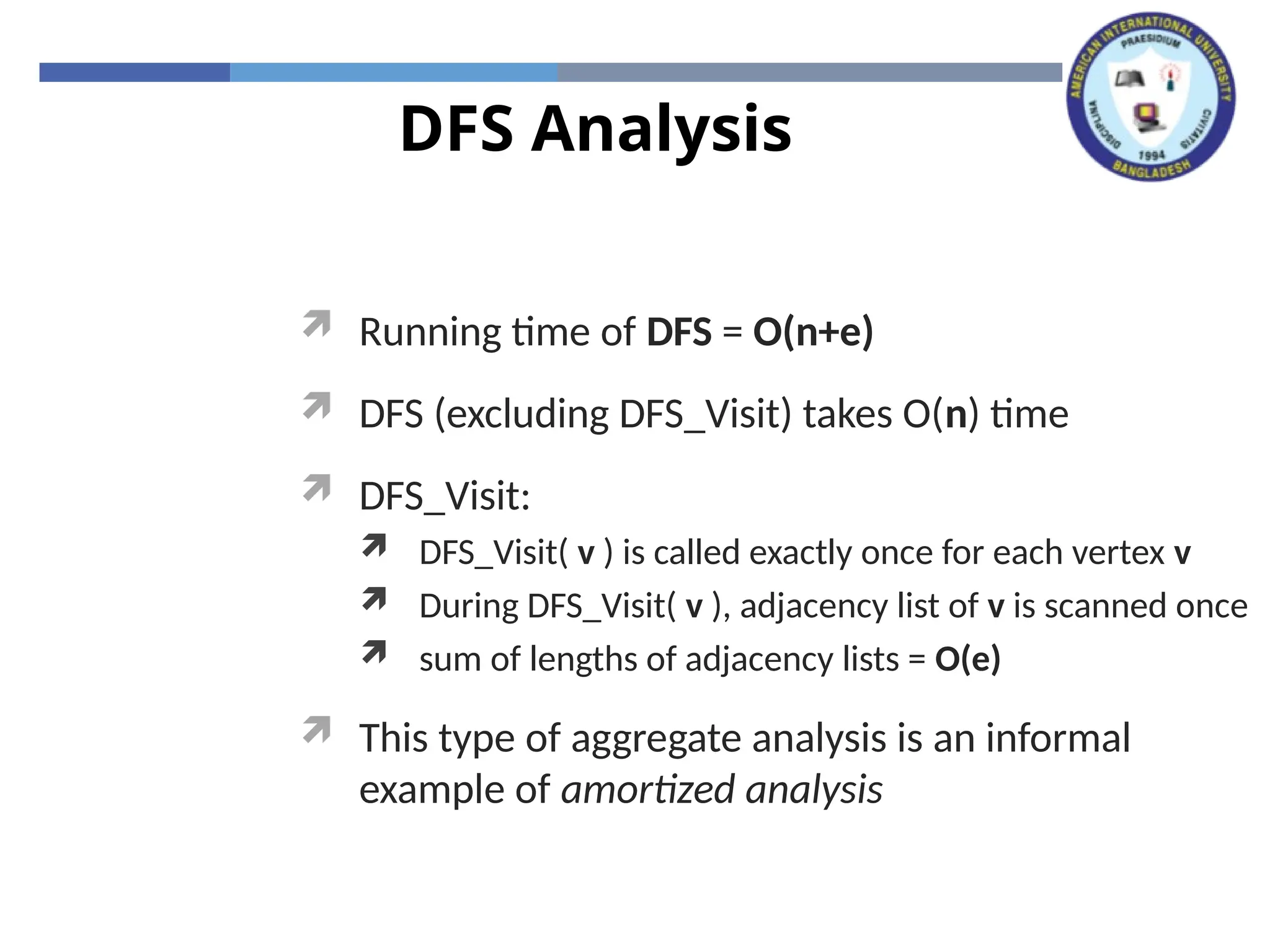
DFS Analysis
Runningtime of DFS = O(n+e)
DFS (excluding DFS_Visit) takes O(n) time
DFS_Visit:
DFS_Visit( v ) is called exactly once for each vertex v
During DFS_Visit( v ), adjacency list of v is scanned once
sum of lengths of adjacency lists = O(e)
This type of aggregate analysis is an informal
example of amortized analysis
44.
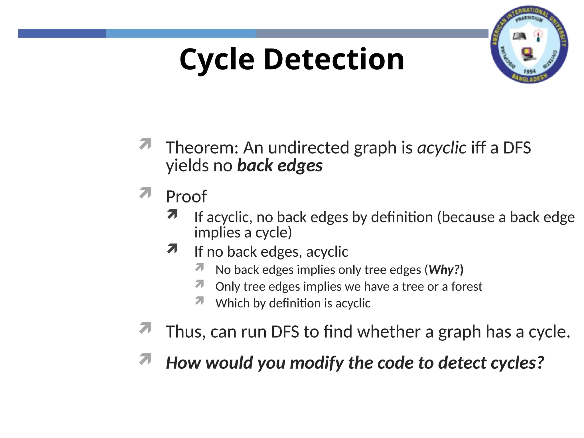
Cycle Detection
Theorem:An undirected graph is acyclic iff a DFS
yields no back edges
Proof
If acyclic, no back edges by definition (because a back edge
implies a cycle)
If no back edges, acyclic
No back edges implies only tree edges (Why?)
Only tree edges implies we have a tree or a forest
Which by definition is acyclic
Thus, can run DFS to find whether a graph has a cycle.
How would you modify the code to detect cycles?
45.
Topological Sort
Finda linear ordering of all vertices of the DAG such that if G
contains an edge (u, v), u appears before v in the ordering.
In general, there may be many legal topological orders for a
given DAG.
Idea:
1. Call DFS(G) to compute finishing time f[ ]
2. Insert vertices onto a linked list according to decreasing order of f[ ]
How to modify DFS to perform Topological Sort in O(n+e) time?
46.
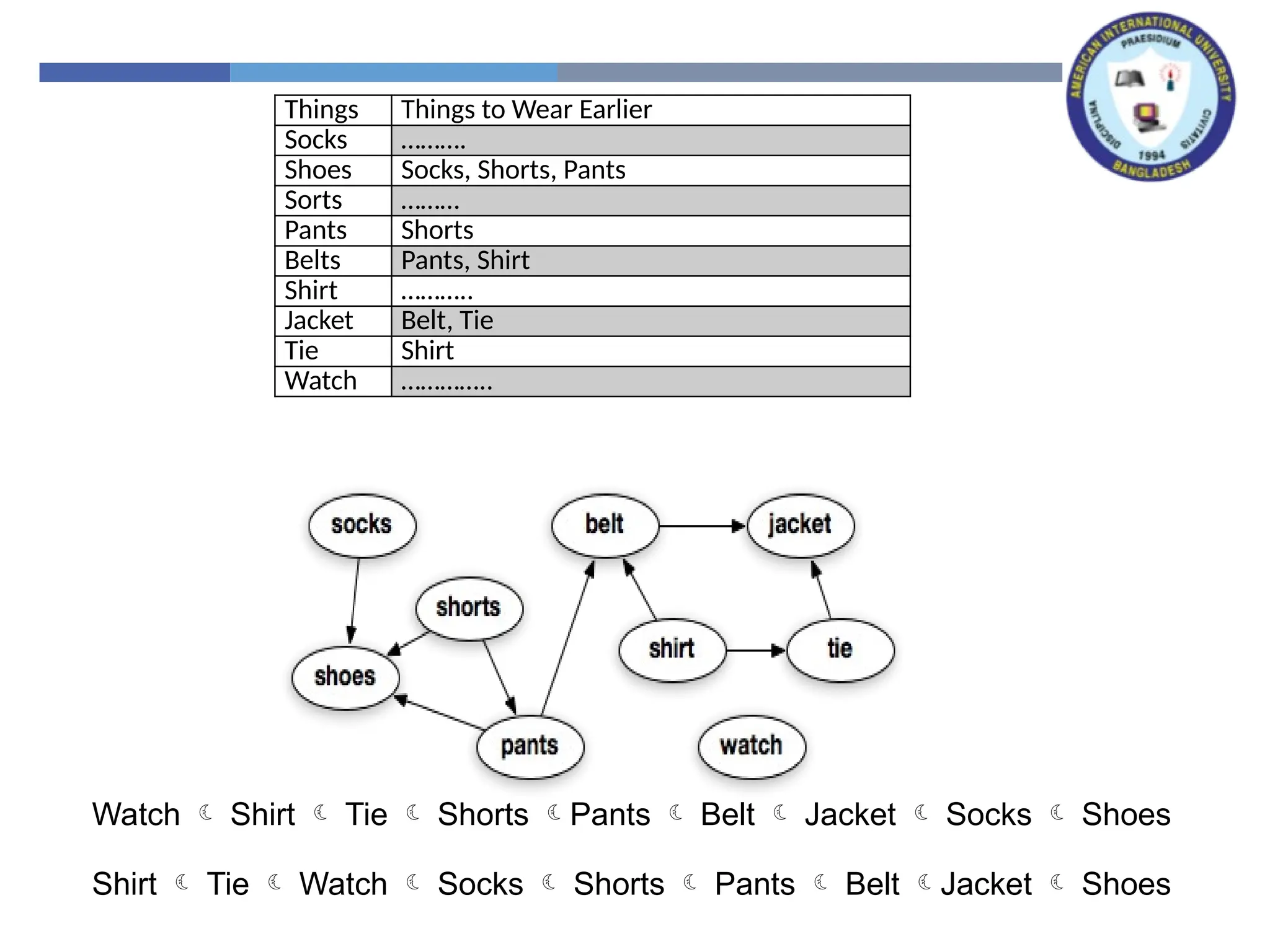
Things Things toWear Earlier
Socks ……….
Shoes Socks, Shorts, Pants
Sorts ………
Pants Shorts
Belts Pants, Shirt
Shirt ………..
Jacket Belt, Tie
Tie Shirt
Watch …………..
Watch Shirt Tie Shorts Pants Belt Jacket Socks Shoes
Shirt Tie Watch Socks Shorts Pants Belt Jacket Shoes
47.
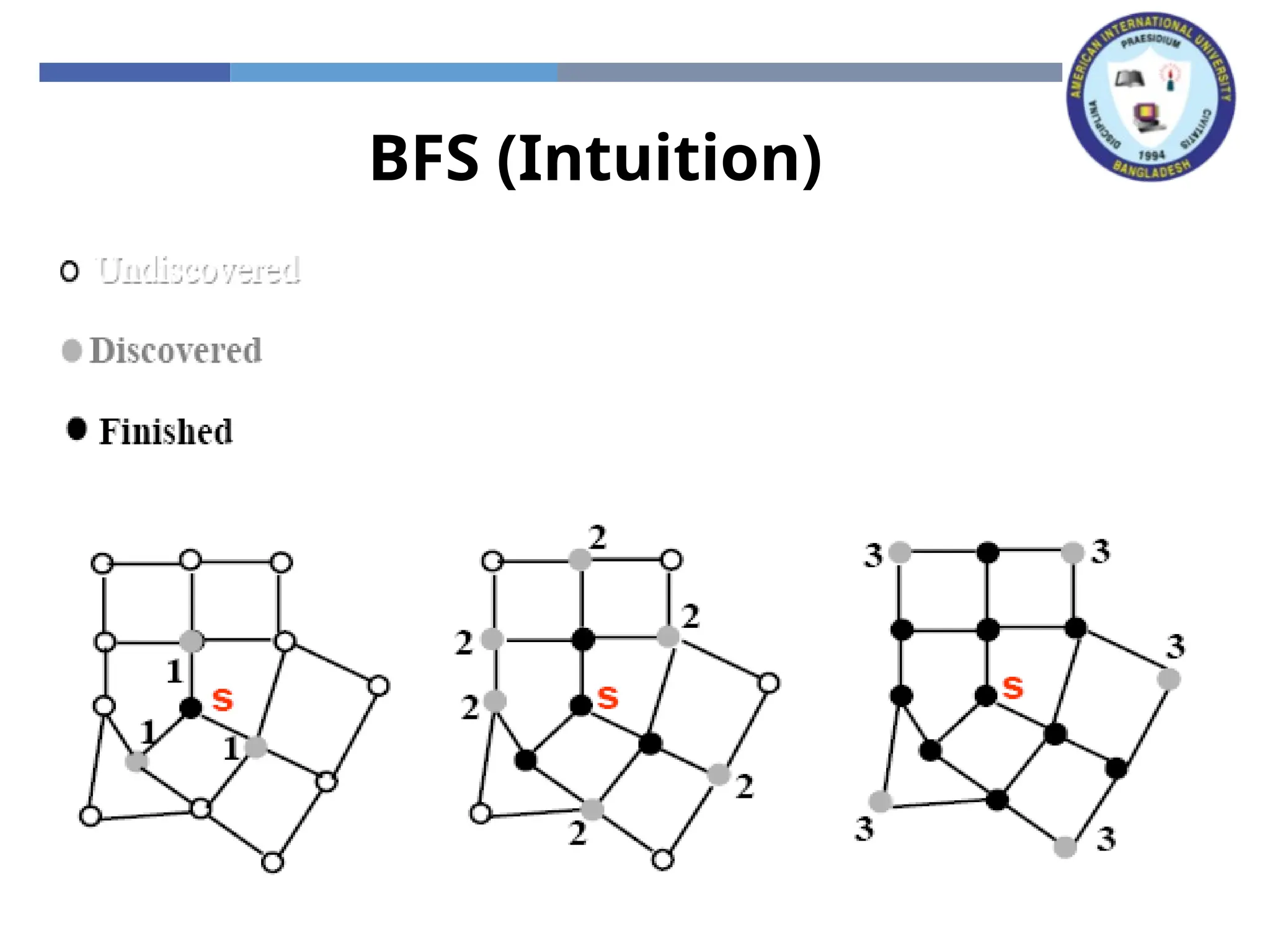
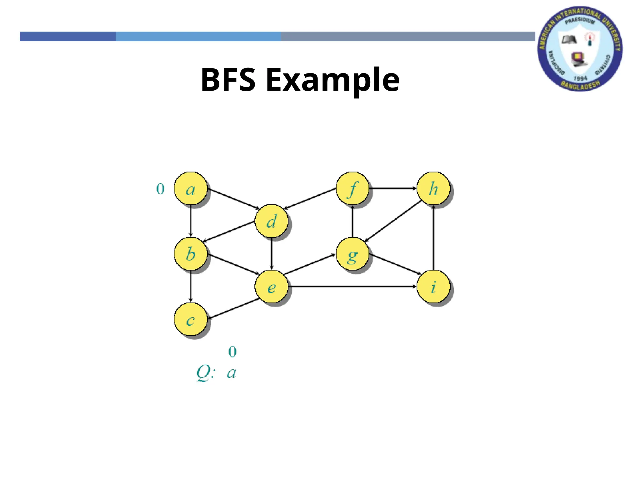
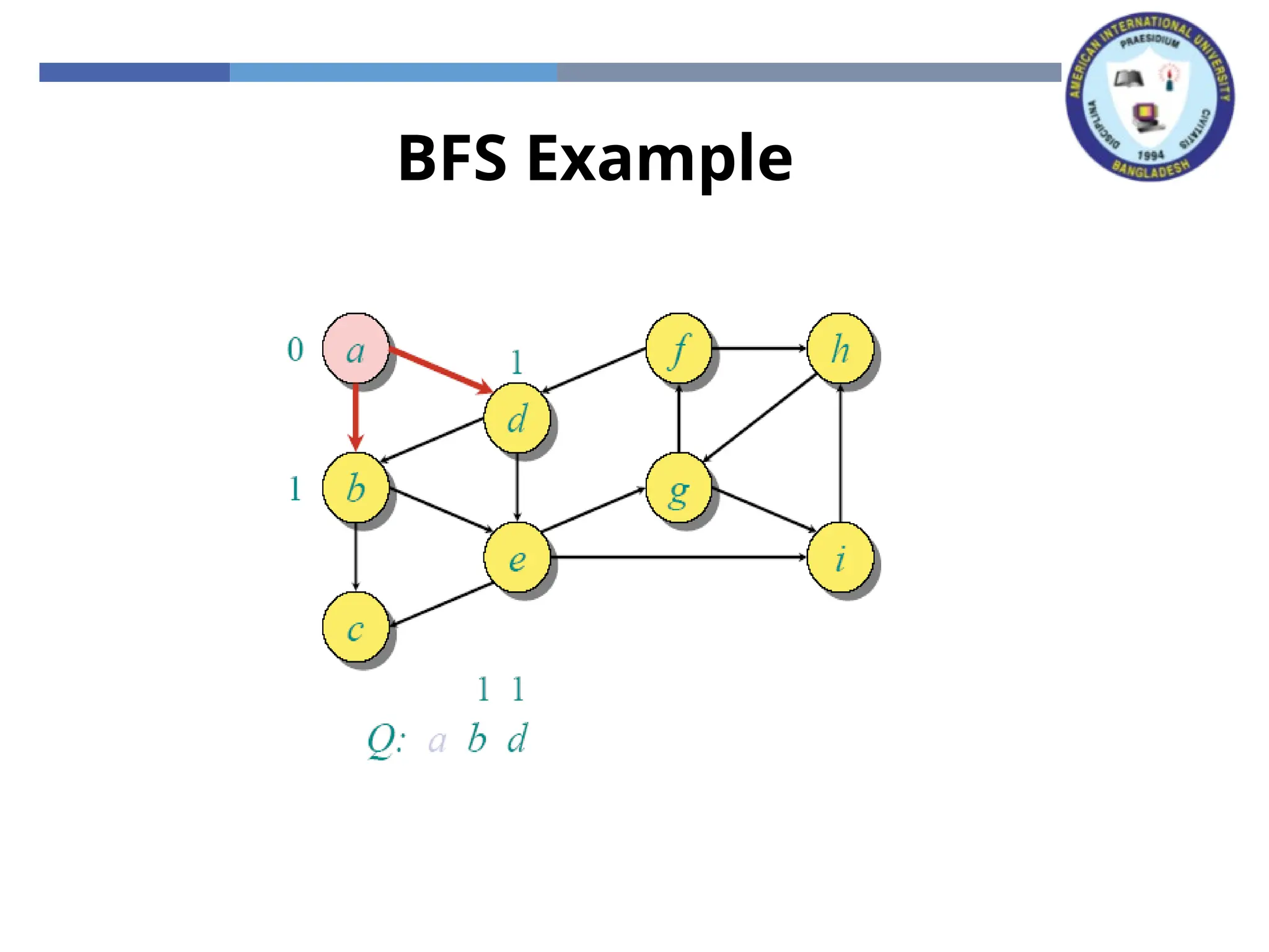
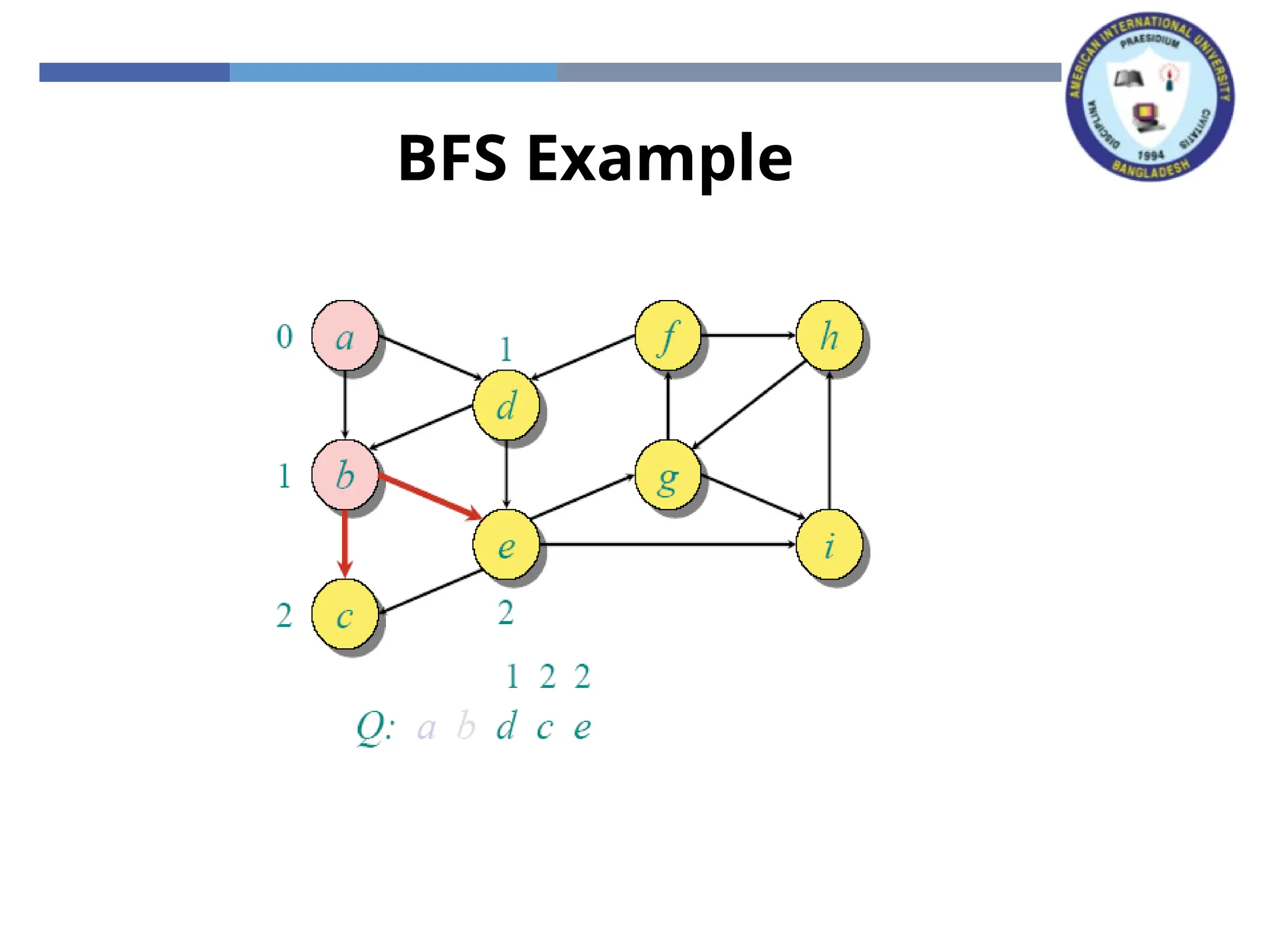
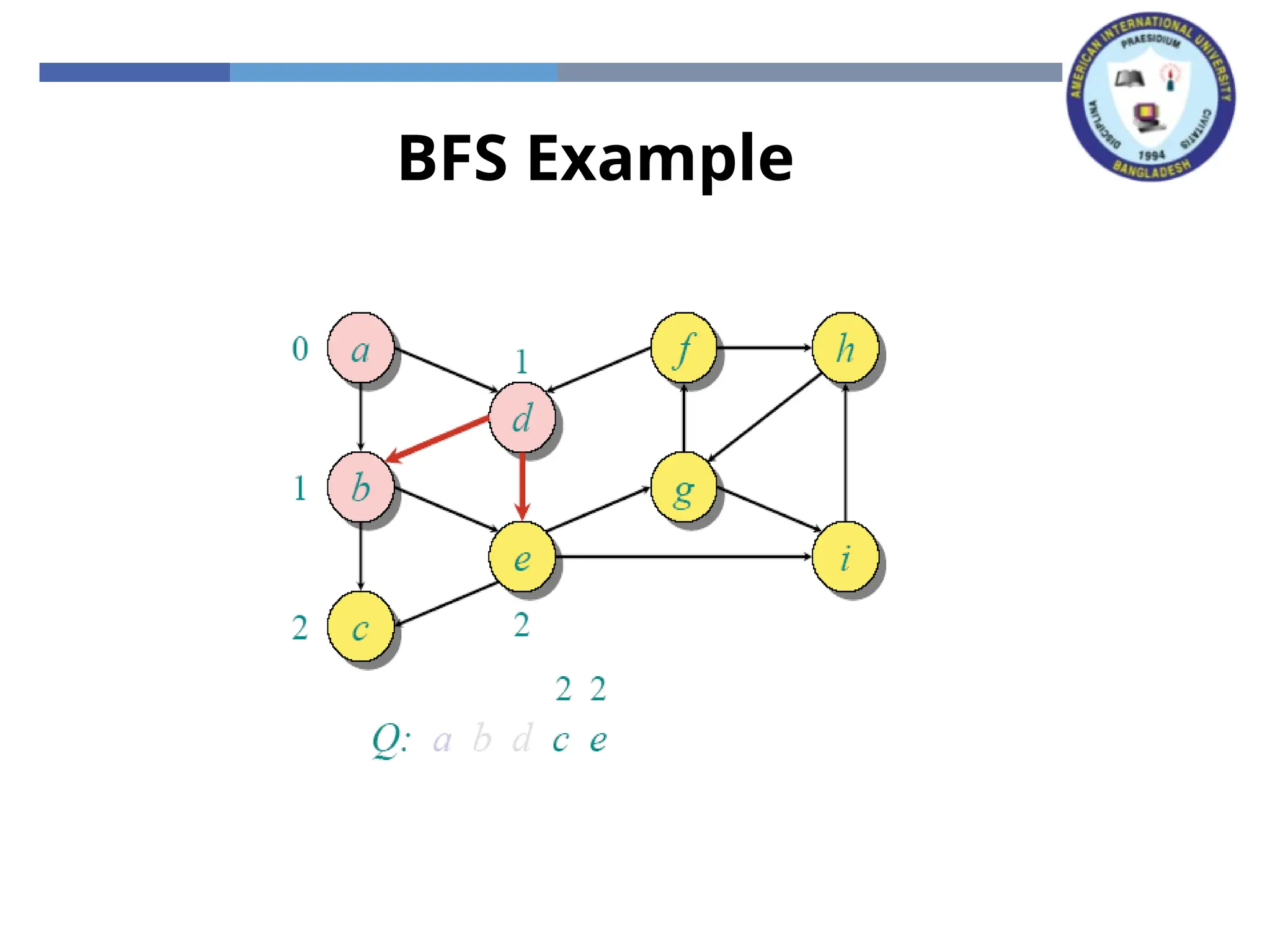
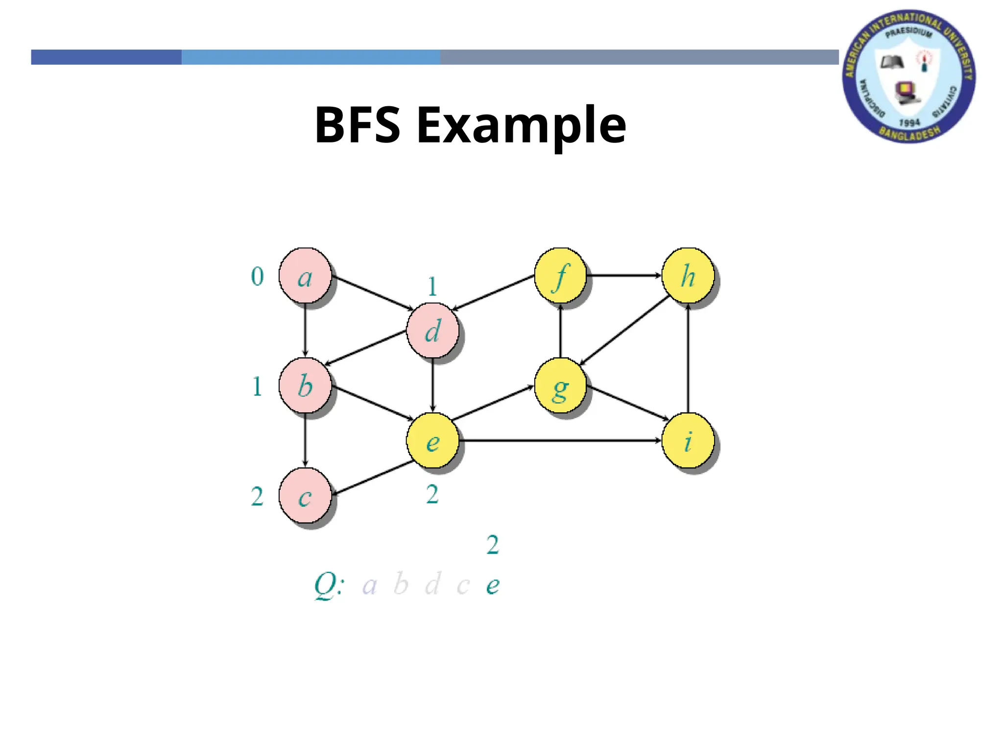
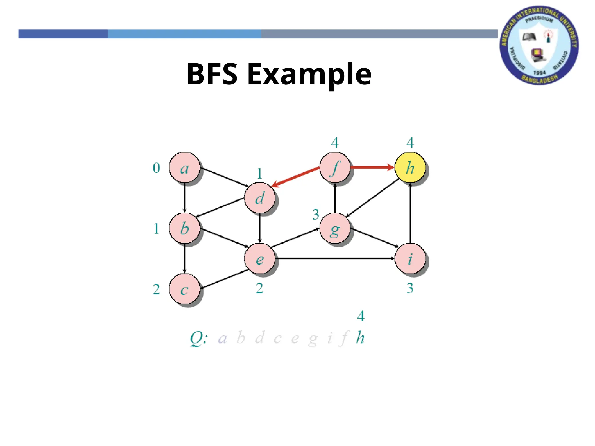
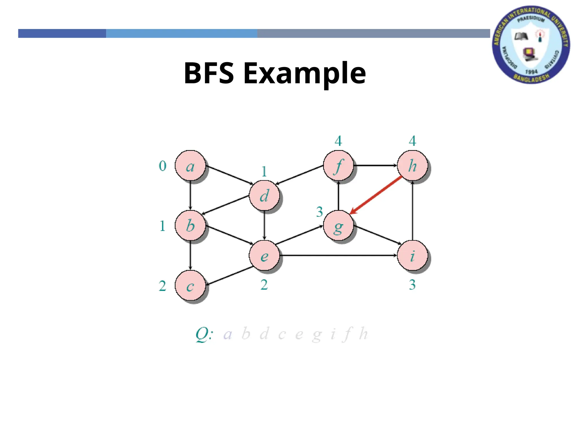
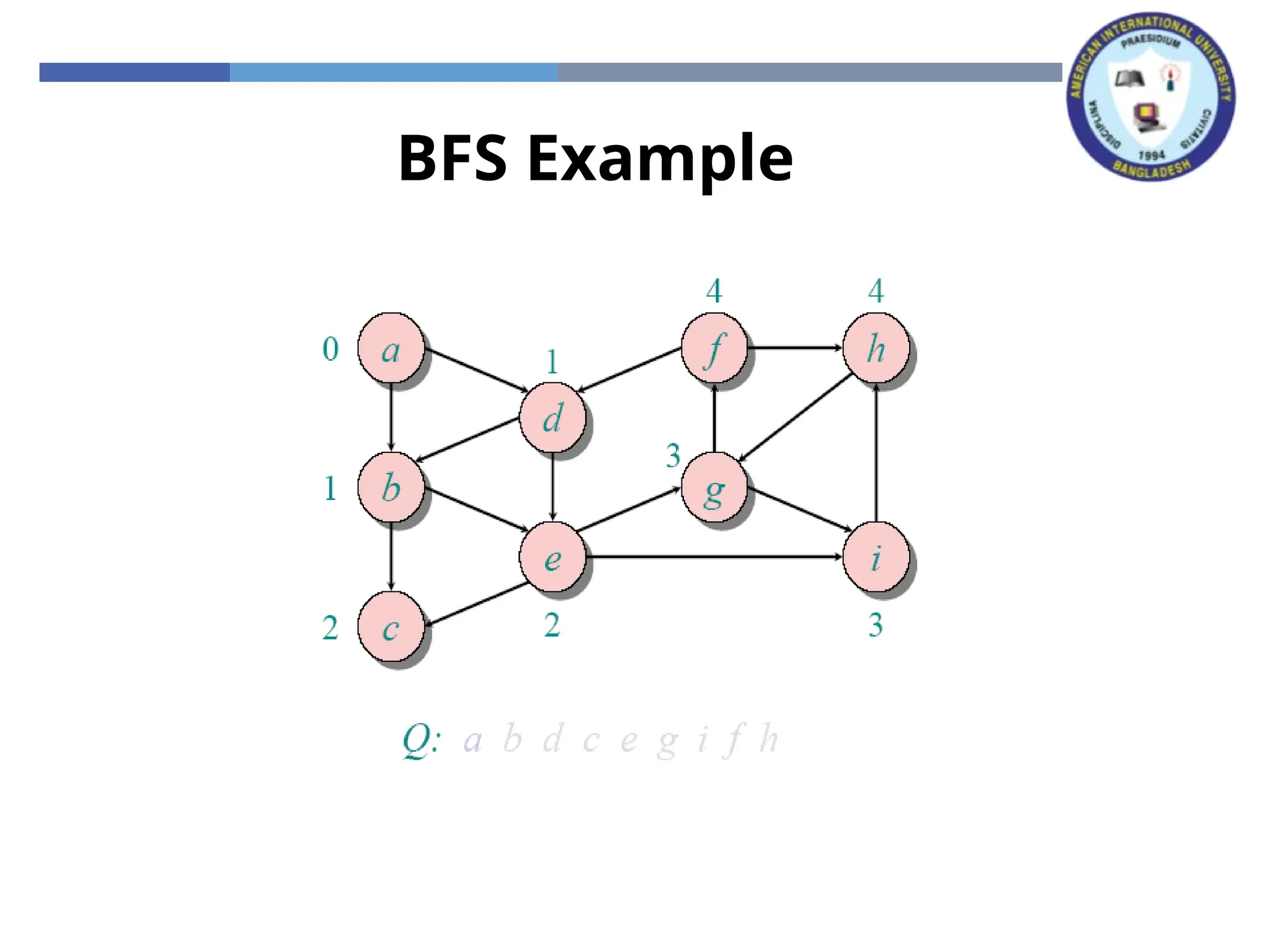
Breadth-First Search (BFS)
Given source vertex s,
systematically explore the breadth of the frontier to
discover every vertex reachable from s
computes the distance d[ ] from s to all reachable vertices
builds a breadth-first tree rooted at s
Algorithm
colors each vertex:
WHITE : undiscovered
GRAY: discovered, in process
BLACK: finished, all adjacent vertices have been discovered
BFS: The Code
BFS(G,s) {
initialize vertices;
Q = {s};
while (Q not empty) {
u = Dequeue(Q);
for each v adjacent to u do {
if (color[v] == WHITE) {
color[v] = GRAY;
d[v] = d[u] + 1;// compute d[]
p[v] = u; // build BFS tree
Enqueue(Q, v);
}
}
color[u] = BLACK;
}
}
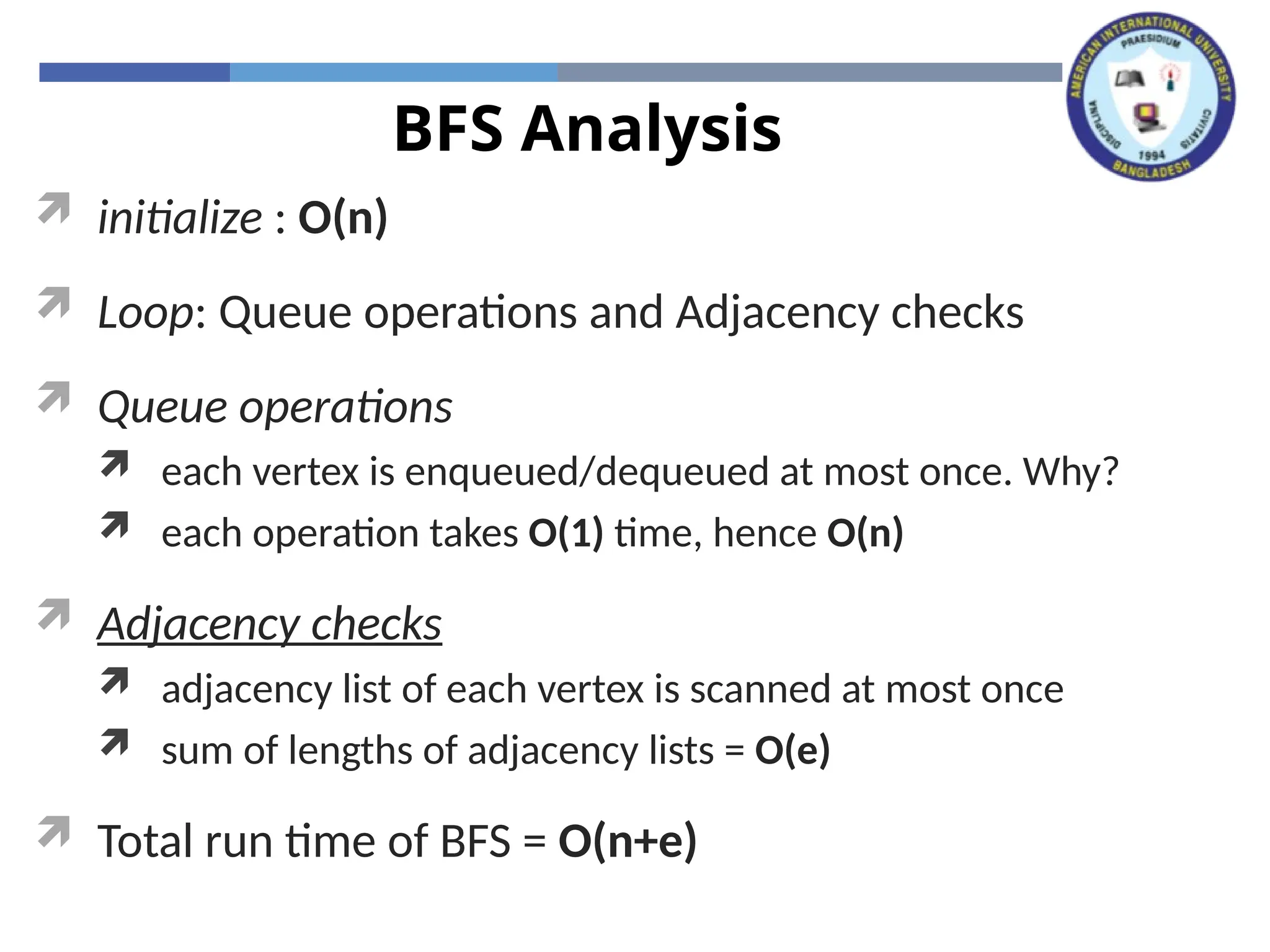
BFS Analysis
initialize: O(n)
Loop: Queue operations and Adjacency checks
Queue operations
each vertex is enqueued/dequeued at most once. Why?
each operation takes O(1) time, hence O(n)
Adjacency checks
adjacency list of each vertex is scanned at most once
sum of lengths of adjacency lists = O(e)
Total run time of BFS = O(n+e)
63.
Breadth-First Search: Properties
What do we get the end of BFS?
1. d[v] = shortest-path distance from s to v, i.e. minimum
number of edges from s to v, or ∞ if v not reachable
from s
Proof : refer CLRS
2. a breadth-first tree, in which path from root s to any
vertex v represent a shortest path
Thus can use BFS to calculate shortest path from one vertex
to another in O(n+e) time, for unweighted graphs.
64.
Books
1. Introduction toAlgorithms, Third Edition, Thomas H. Cormen, Charle E. Leiserson,
Ronald L. Rivest, Clifford Stein (CLRS).
2. Fundamental of Computer Algorithms, Ellis Horowitz, Sartaj Sahni, Sanguthevar
Rajasekaran (HSR)
#8 A dense graph is one where there are many edges, but not necessarily as many as in a complete graph. This term is intentionally vague and is intended to convey a general sense that the number of edges can be expected to be large with respect to the number of vertices.


![Graph Representation
Adjacency matrix: represents a graph as n x n matrix A (here, n is
the number of nodes/ vertices):
A[i, j] = 1 if edge (i, j) E (or weight of edge)
= 0 if edge (i, j) E
Storage requirements: O(n2
)
Using adjacency matrix is more efficient to represent dense
graphs
Especially if store just one bit/edge
Undirected graph: only need half of matrix](https://image.slidesharecdn.com/week10graphsandtrees-251204165730-d8b224db/75/ProgrammingProgramming-Graphs-and-Trees-pptx-15-2048.jpg)
![Depth-First Search (DFS)
Explore “deeper” in the graph whenever possible
Edges are explored out of the most recently discovered vertex v that still has
unexplored edges (LIFO)
When all of v’s edges have been explored, backtrack to the vertex from which
v was discovered
computes 2 timestamps: d[ ] (discovered) and f[ ] (finished)
builds one or more depth-first tree(s) (depth-first forest)
Algorithm colors each vertex
WHITE: undiscovered
GRAY: discovered, in process
BLACK: finished, all adjacent vertices have been discovered](https://image.slidesharecdn.com/week10graphsandtrees-251204165730-d8b224db/75/ProgrammingProgramming-Graphs-and-Trees-pptx-23-2048.jpg)
![Depth-First Search: The Code
DFS(G)
{
for each vertex u V
color[u] = WHITE;
time = 0;
for each vertex u V
if (color[u] == WHITE)
DFS_Visit(u);
}
DFS_Visit(u)
{
color[u] = GREY;
time = time+1;
d[u] = time; // compute d[]
for each v adjacent to u
if (color[v] == WHITE)
p[v]= u // build tree
DFS_Visit(v);
color[u] = BLACK;
time = time+1;
f[u] = time; // compute f[]
}
](https://image.slidesharecdn.com/week10graphsandtrees-251204165730-d8b224db/75/ProgrammingProgramming-Graphs-and-Trees-pptx-24-2048.jpg)


![Topological Sort
Find a linear ordering of all vertices of the DAG such that if G
contains an edge (u, v), u appears before v in the ordering.
In general, there may be many legal topological orders for a
given DAG.
Idea:
1. Call DFS(G) to compute finishing time f[ ]
2. Insert vertices onto a linked list according to decreasing order of f[ ]
How to modify DFS to perform Topological Sort in O(n+e) time?](https://image.slidesharecdn.com/week10graphsandtrees-251204165730-d8b224db/75/ProgrammingProgramming-Graphs-and-Trees-pptx-45-2048.jpg)
![Breadth-First Search (BFS)
Given source vertex s,
systematically explore the breadth of the frontier to
discover every vertex reachable from s
computes the distance d[ ] from s to all reachable vertices
builds a breadth-first tree rooted at s
Algorithm
colors each vertex:
WHITE : undiscovered
GRAY: discovered, in process
BLACK: finished, all adjacent vertices have been discovered](https://image.slidesharecdn.com/week10graphsandtrees-251204165730-d8b224db/75/ProgrammingProgramming-Graphs-and-Trees-pptx-47-2048.jpg)
![BFS: The Code
BFS(G, s) {
initialize vertices;
Q = {s};
while (Q not empty) {
u = Dequeue(Q);
for each v adjacent to u do {
if (color[v] == WHITE) {
color[v] = GRAY;
d[v] = d[u] + 1;// compute d[]
p[v] = u; // build BFS tree
Enqueue(Q, v);
}
}
color[u] = BLACK;
}
}](https://image.slidesharecdn.com/week10graphsandtrees-251204165730-d8b224db/75/ProgrammingProgramming-Graphs-and-Trees-pptx-49-2048.jpg)
![Breadth-First Search: Properties
What do we get the end of BFS?
1. d[v] = shortest-path distance from s to v, i.e. minimum
number of edges from s to v, or ∞ if v not reachable
from s
Proof : refer CLRS
2. a breadth-first tree, in which path from root s to any
vertex v represent a shortest path
Thus can use BFS to calculate shortest path from one vertex
to another in O(n+e) time, for unweighted graphs.](https://image.slidesharecdn.com/week10graphsandtrees-251204165730-d8b224db/75/ProgrammingProgramming-Graphs-and-Trees-pptx-63-2048.jpg)