
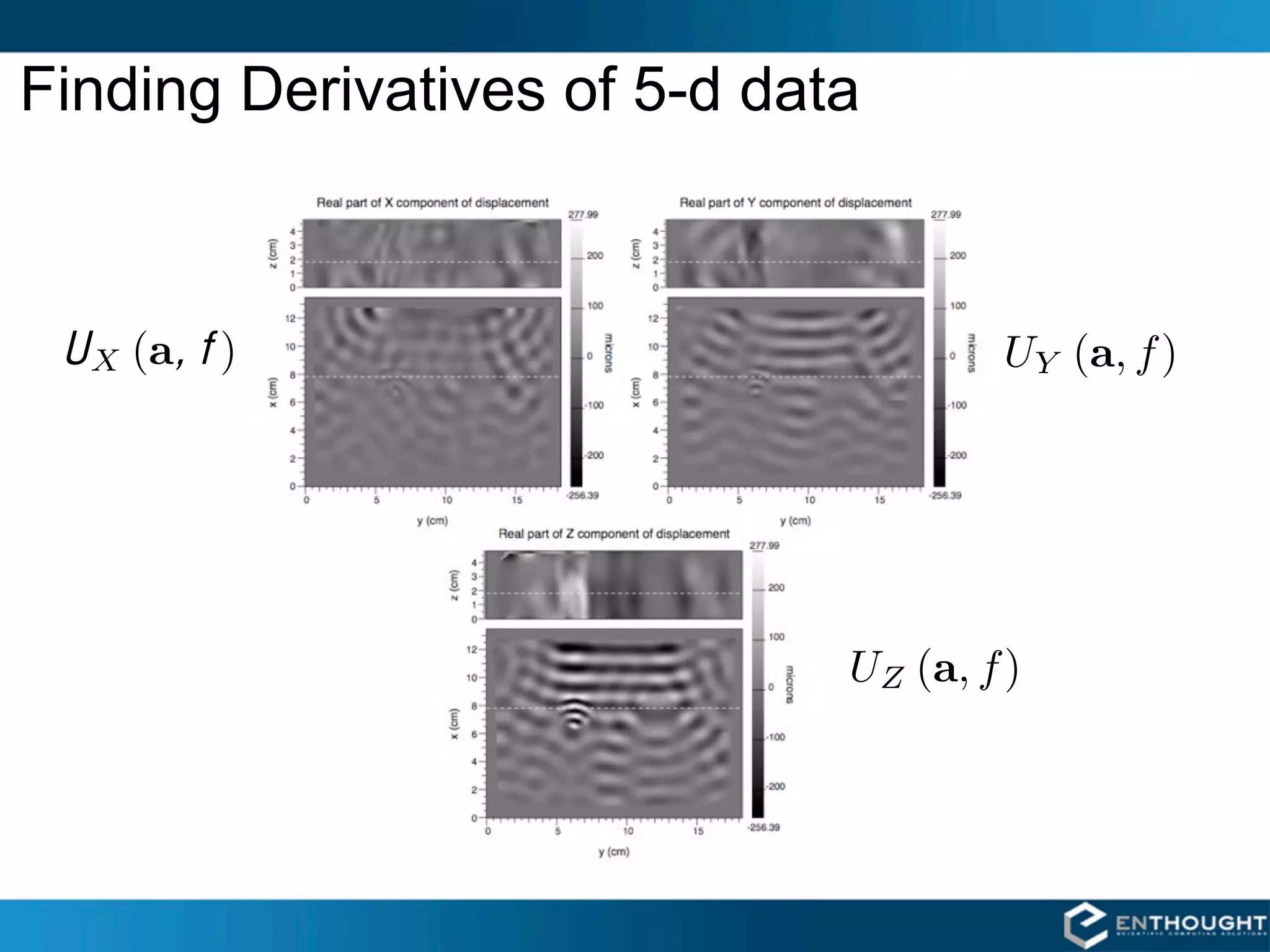
![Magnetic Resonance Elastography 1997
Richard Ehman
Armando Manduca
Raja Muthupillai
2
ρ0 (2πf ) Ui (a, f ) = [Cijkl (a, f ) Uk,l (a, f )],j](https://image.slidesharecdn.com/numpytalksiam-110305000848-phpapp01/75/Numpy-Talk-at-SIAM-2-2048.jpg)
![SciPy [ Scientific Algorithms ]
linalg stats interpolate
cluster special maxentropy
io fftpack odr
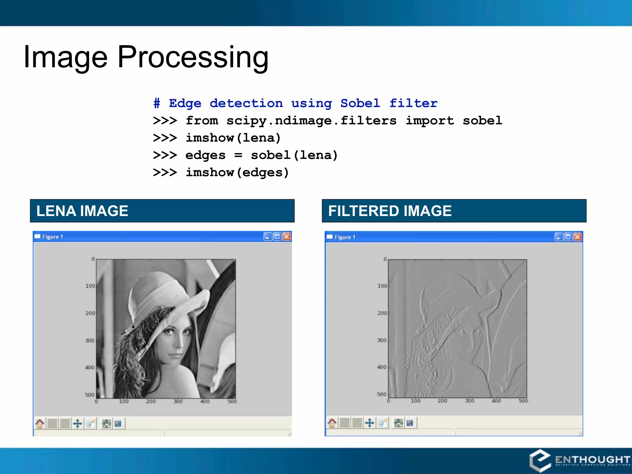
ndimage sparse integrate
signal optimize weave
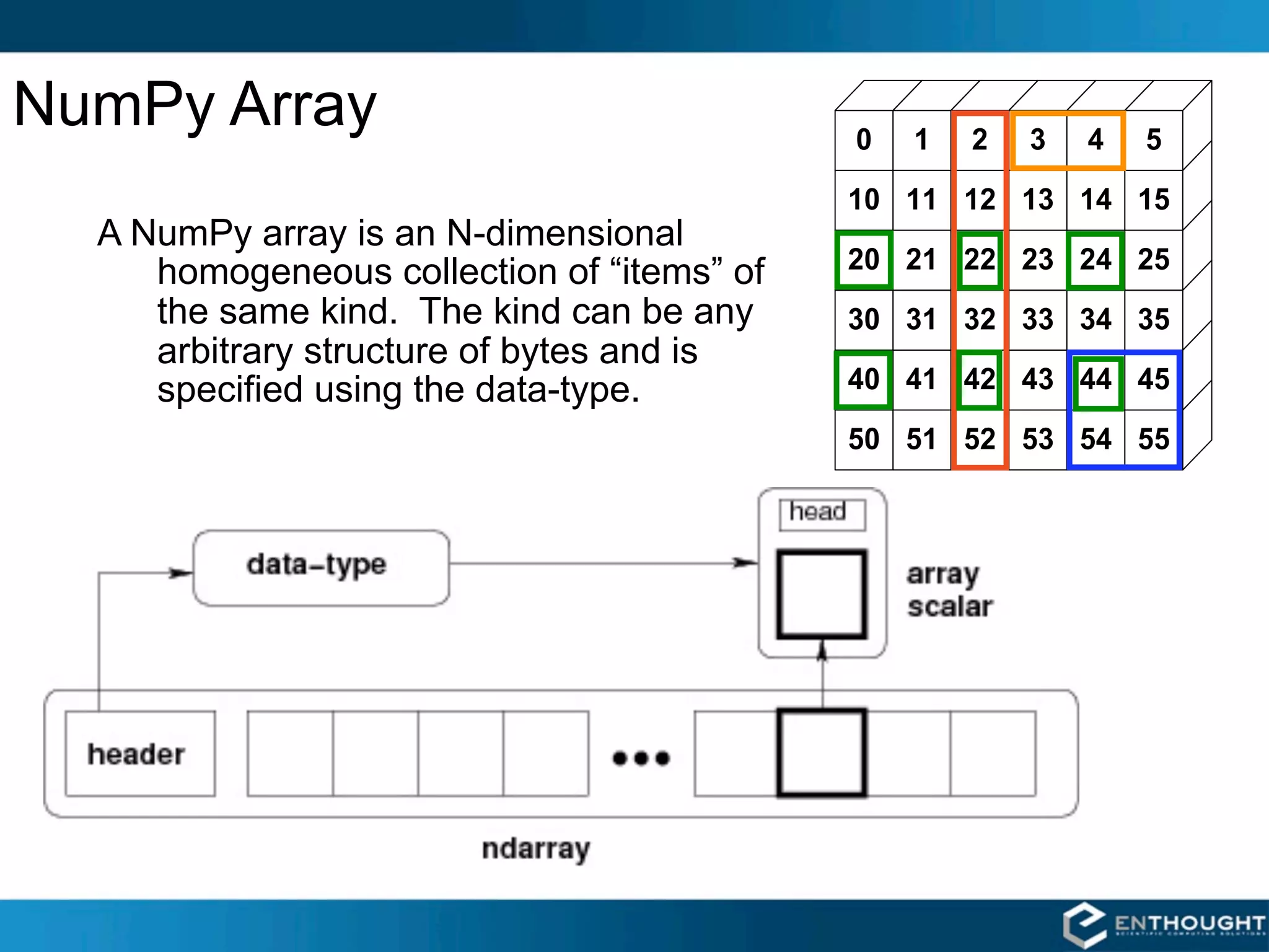
NumPy [ Data Structure Core ]
fft random linalg
NDArray UFunc
multi-dimensional fast array
array object math operations
Python](https://image.slidesharecdn.com/numpytalksiam-110305000848-phpapp01/75/Numpy-Talk-at-SIAM-6-2048.jpg)


![Optimization: Data Fitting
NONLINEAR LEAST SQUARES CURVE FITTING
>>> from scipy.optimize import curve_fit
>>> from scipy.stats import norm
# Define the function to fit.
>>> def function(x, a , b, f, phi):
... result = a * exp(-b * sin(f * x + phi))
... return result
# Create a noisy data set.
>>> actual_params = [3, 2, 1, pi/4]
>>> x = linspace(0,2*pi,25)
>>> exact = function(x, *actual_params)
>>> noisy = exact + 0.3*norm.rvs(size=len(x))
# Use curve_fit to estimate the function parameters from the noisy data.
>>> initial_guess = [1,1,1,1]
>>> estimated_params, err_est = curve_fit(function, x, noisy, p0=initial_guess)
>>> estimated_params
array([3.1705, 1.9501, 1.0206, 0.7034])
# err_est is an estimate of the covariance matrix of the estimates
# (i.e. how good of a fit is it)](https://image.slidesharecdn.com/numpytalksiam-110305000848-phpapp01/75/Numpy-Talk-at-SIAM-9-2048.jpg)
![2D RBF Interpolation
EXAMPLE
>>> from scipy.interpolate import
... Rbf
>>> from numpy import hypot, mgrid
>>> from scipy.special import j0
>>> x, y = mgrid[-5:6,-5:6]
>>> z = j0(hypot(x,y))
>>> newfunc = Rbf(x, y, z)
>>> xx, yy = mgrid[-5:5:100j,
-5:5:100j]
# xx and yy are both 2-d
# result is evaluated
# element-by-element
>>> zz = newfunc(xx, yy)
>>> from enthought.mayavi import mlab
>>> mlab.surf(x, y, z*5)
>>> mlab.figure()
>>> mlab.surf(xx, yy, zz*5)
>>> mlab.points3d(x,y,z*5,
scale_factor=0.5)](https://image.slidesharecdn.com/numpytalksiam-110305000848-phpapp01/75/Numpy-Talk-at-SIAM-10-2048.jpg)
![Brownian Motion
Brownian motion (Wiener process):
2
X (t + dt) = X (t) + N 0, σ dt, t, t + dt
where N (a, b, t1 , t2 ) is normal with mean a
and variance b, and independent on
disjoint time intervals.
>>> from scipy.stats import norm
>>> x0 = 100.0
>>> dt = 0.5
>>> sigma = 1.5
>>> n = 100
>>> steps = norm.rvs(size=n,
scale=sigma*sqrt(dt))
>>> steps[0] = x0 # Make i.c. work
>>> x = steps.cumsum()
>>> t = linspace(0, (n-1)*dt, n)
>>> plot(t, x)](https://image.slidesharecdn.com/numpytalksiam-110305000848-phpapp01/75/Numpy-Talk-at-SIAM-11-2048.jpg)
![Array Slicing
SLICING WORKS MUCH LIKE
STANDARD PYTHON SLICING
>>> a[0,3:5]
array([3, 4])
>>> a[4:,4:]
array([[44, 45],
[54, 55]])
>>> a[:,2]
array([2,12,22,32,42,52])
STRIDES ARE ALSO POSSIBLE
>>> a[2::2,::2]
array([[20, 22, 24],
[40, 42, 44]])
14](https://image.slidesharecdn.com/numpytalksiam-110305000848-phpapp01/75/Numpy-Talk-at-SIAM-14-2048.jpg)
![Fancy Indexing in 2-D
>>> a[(0,1,2,3,4),(1,2,3,4,5)]
array([ 1, 12, 23, 34, 45])
>>> a[3:,[0, 2, 5]]
array([[30, 32, 35],
[40, 42, 45],
[50, 52, 55]])
>>> mask = array([1,0,1,0,0,1],
dtype=bool)
>>> a[mask,2]
array([2,22,52])
Unlike slicing, fancy indexing
creates copies instead of a
view into original array.](https://image.slidesharecdn.com/numpytalksiam-110305000848-phpapp01/75/Numpy-Talk-at-SIAM-15-2048.jpg)
![Fancy Indexing with Indices
INDEXING BY POSITION
# create an Nx3 colormap
# grayscale map -- R G B
>>> cmap = array([[1.0,1.0,1.0],
[0.9,0.9,0.9],
...
[0.0,0.0,0.0]])
>>> cmap.shape
(10,3)
>>> img = array([[0,10],
[5,1 ]])
>>> img.shape
(2,2)
# use the image as an index into
# the colormap
>>> rgb_img = cmap[img]
>>> rgb_img.shape
(2,2,3)
16](https://image.slidesharecdn.com/numpytalksiam-110305000848-phpapp01/75/Numpy-Talk-at-SIAM-16-2048.jpg)
![“Structured” Arrays
Elements of an array can be EXAMPLE
any fixed-size data structure! >>> from numpy import dtype, empty
# structured data format
name char[10] >>> fmt = dtype([('name', 'S10'),
age int ('age', int),
weight double ('weight', float)
])
>>> a = empty((3,4), dtype=fmt)
Brad Jane John Fred >>> a.itemsize
22
33 25 47 54
>>> a['name'] = [['Brad', … ,'Jill']]
135.0 105.0 225.0 140.0 >>> a['age'] = [[33, … , 54]]
Henry George Brian Amy >>> a['weight'] = [[135, … , 145]]
>>> print a
29 61 32 27 [[('Brad', 33, 135.0)
154.0 202.0 137.0 187.0 …
Ron Susan Jennifer Jill
('Jill', 54, 145.0)]]
19 33 18 54
188.0 135.0 88.0 145.0](https://image.slidesharecdn.com/numpytalksiam-110305000848-phpapp01/75/Numpy-Talk-at-SIAM-19-2048.jpg)
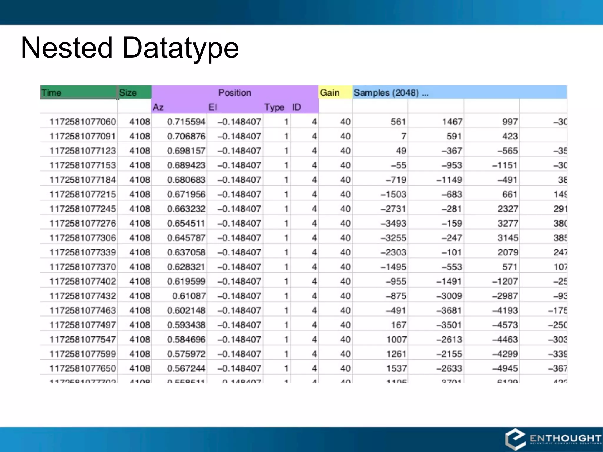
![Nested Datatype
dt = dtype([('time', uint64),
('size', uint32),
('position', [('az', float32),
('el', float32),
('region_type', uint8),
('region_ID', uint16)]),
('gain', np.uint8),
('samples', np.int16, 2048)])
data = np.fromfile(f, dtype=dt)](https://image.slidesharecdn.com/numpytalksiam-110305000848-phpapp01/75/Numpy-Talk-at-SIAM-21-2048.jpg)

![Structured Arrays
char[12] int64 float32 Elements of array can be any
fixed-size data structure!
Name Time Value
MSFT_profit 10 6.20 Example
GOOG_profit 12 -1.08 >>> import numpy as np
>>> fmt = np.dtype([('name', 'S12'),
MSFT_profit 18 8.40 ('time', np.int64),
('value', np.float32)])
>>> vals = [('MSFT_profit', 10, 6.20),
INTC_profit 25 -0.20 ('GOOG_profit', 12, -1.08),
…
('INTC_profit', 1000385, -1.05)
('MSFT_profit', 1000390, 5.60)]
GOOG_profit 1000325 3.20
>>> arr = np.array(vals, dtype=fmt)
GOOG_profit 1000350 4.50 # or
>>> arr = np.fromfile('db.dat', dtype=fmt)
INTC_profit 1000385 -1.05 # or
>>> arr = np.memmap('db.dat', dtype=fmt,
mode='c')
MSFT_profit 1000390 5.60
MSFT_profit 10 6.20 GOOG_profit 12 -1.08 INTC_profit 1000385 -1.05 MSFT_profit 1000390 5.60](https://image.slidesharecdn.com/numpytalksiam-110305000848-phpapp01/75/Numpy-Talk-at-SIAM-24-2048.jpg)
![Mathematical Binary Operators
a + b add(a,b) a * b multiply(a,b)
a - b subtract(a,b) a / b divide(a,b)
a % b remainder(a,b) a ** b power(a,b)
MULTIPLY BY A SCALAR ADDITION USING AN OPERATOR
FUNCTION
>>> a = array((1,2))
>>> a*3. >>> add(a,b)
array([3., 6.]) array([4, 6])
ELEMENT BY ELEMENT ADDITION IN-PLACE OPERATION
# Overwrite contents of a.
>>> a = array([1,2])
# Saves array creation
>>> b = array([3,4])
# overhead.
>>> a + b
>>> add(a,b,a) # a += b
array([4, 6])
array([4, 6])
>>> a
array([4, 6])](https://image.slidesharecdn.com/numpytalksiam-110305000848-phpapp01/75/Numpy-Talk-at-SIAM-25-2048.jpg)
![Comparison and Logical Operators
equal (==) not_equal (!=) greater (>)
greater_equal (>=) less (<) less_equal (<=)
logical_and logical_or logical_xor
logical_not
2-D EXAMPLE
Be careful with if statements
>>> a = array(((1,2,3,4),(2,3,4,5))) involving numpy arrays. To
>>> b = array(((1,2,5,4),(1,3,4,5))) test for equality of arrays,
>>> a == b don't do:
array([[True, True, False, True], if a == b:
[False, True, True, True]])
# functional equivalent Rather, do:
>>> equal(a,b) if all(a==b):
array([[True, True, False, True],
[False, True, True, True]]) For floating point,
if allclose(a,b):
is even better.](https://image.slidesharecdn.com/numpytalksiam-110305000848-phpapp01/75/Numpy-Talk-at-SIAM-26-2048.jpg)
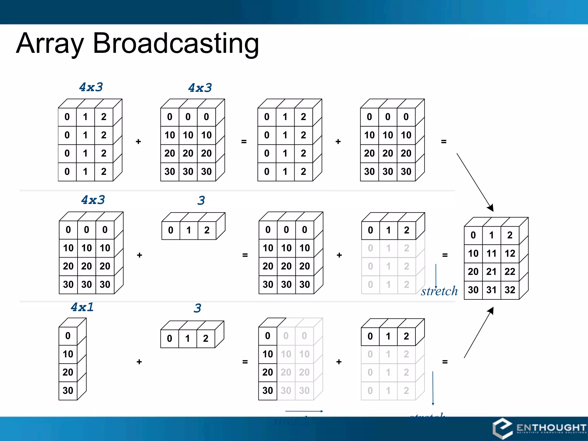
![Broadcasting in Action
>>> a = array((0,10,20,30))
>>> b = array((0,1,2))
>>> y = a[:, newaxis] + b](https://image.slidesharecdn.com/numpytalksiam-110305000848-phpapp01/75/Numpy-Talk-at-SIAM-29-2048.jpg)
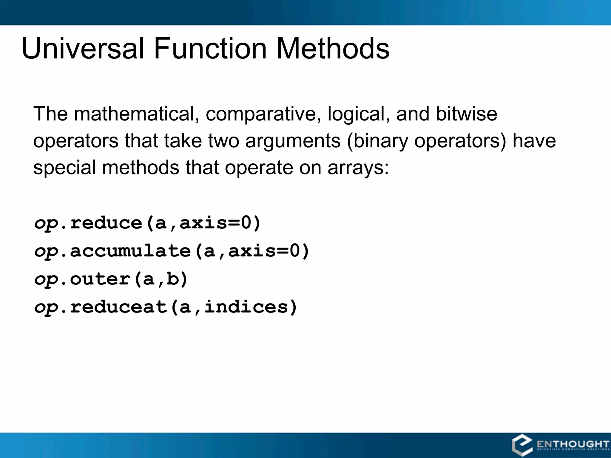
![op.reduce()
For multidimensional arrays, op.reduce(a,axis)applies op to the elements of a
along the specified axis. The resulting array has dimensionality one less than a. The
default value for axis is 0.
SUM COLUMNS BY DEFAULT SUMMING UP EACH ROW
>>> add.reduce(a) >>> add.reduce(a,1)
array([60, 64, 68]) array([ 3, 33, 63, 93])](https://image.slidesharecdn.com/numpytalksiam-110305000848-phpapp01/75/Numpy-Talk-at-SIAM-31-2048.jpg)
![Array Calculation Methods
SUM FUNCTION SUM ARRAY METHOD
>>> a = array([[1,2,3], # a.sum() defaults to adding
[4,5,6]], float) # up all values in an array.
>>> a.sum()
# sum() defaults to adding up 21.
# all the values in an array.
>>> sum(a) # supply an axis argument to
21. # sum along a specific axis
>>> a.sum(axis=0)
# supply the keyword axis to array([5., 7., 9.])
# sum along the 0th axis
>>> sum(a, axis=0)
array([5., 7., 9.]) PRODUCT
# product along columns
# supply the keyword axis to >>> a.prod(axis=0)
# sum along the last axis array([ 4., 10., 18.])
>>> sum(a, axis=-1)
array([6., 15.]) # functional form
>>> prod(a, axis=0)
array([ 4., 10., 18.])](https://image.slidesharecdn.com/numpytalksiam-110305000848-phpapp01/75/Numpy-Talk-at-SIAM-32-2048.jpg)
![Min/Max
MIN MAX
>>> a = array([2.,3.,0.,1.]) >>> a = array([2.,3.,0.,1.])
>>> a.min(axis=0) >>> a.max(axis=0)
0. 3.
# Use NumPy's amin() instead
# of Python's built-in min()
# for speedy operations on
# multi-dimensional arrays. # functional form
>>> amin(a, axis=0) >>> amax(a, axis=0)
0. 3.
ARGMIN ARGMAX
# Find index of minimum value. # Find index of maximum value.
>>> a.argmin(axis=0) >>> a.argmax(axis=0)
2 1
# functional form # functional form
>>> argmin(a, axis=0) >>> argmax(a, axis=0)
2 1](https://image.slidesharecdn.com/numpytalksiam-110305000848-phpapp01/75/Numpy-Talk-at-SIAM-33-2048.jpg)
![Statistics Array Methods
MEAN STANDARD DEV./VARIANCE
>>> a = array([[1,2,3], # Standard Deviation
[4,5,6]], float) >>> a.std(axis=0)
array([ 1.5, 1.5, 1.5])
# mean value of each column
>>> a.mean(axis=0) # variance
array([ 2.5, 3.5, 4.5]) >>> a.var(axis=0)
>>> mean(a, axis=0) array([2.25, 2.25, 2.25])
array([ 2.5, 3.5, 4.5]) >>> var(a, axis=0)
>>> average(a, axis=0) array([2.25, 2.25, 2.25])
array([ 2.5, 3.5, 4.5])
# average can also calculate
# a weighted average
>>> average(a, weights=[1,2],
... axis=0)
array([ 3., 4., 5.])](https://image.slidesharecdn.com/numpytalksiam-110305000848-phpapp01/75/Numpy-Talk-at-SIAM-34-2048.jpg)


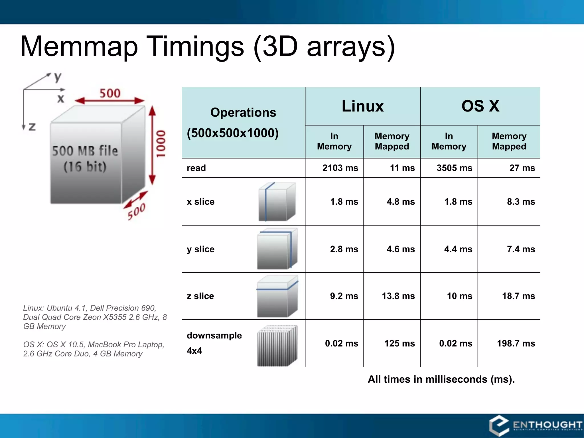
SciPy and NumPy are Python packages that provide scientific computing capabilities. NumPy provides multidimensional array objects and fast linear algebra functions. SciPy builds on NumPy and adds modules for optimization, integration, signal and image processing, and more. Together, NumPy and SciPy give Python powerful data analysis and visualization capabilities. The community contributes to both projects to expand their functionality. Memory mapped arrays in NumPy allow working with large datasets that exceed system memory.


![Coded Agents – with UiPath SDK + LangGraph [Virtual Hands-on Workshop]](https://cdn.slidesharecdn.com/ss_thumbnails/codedagentsdeck-251215155422-5497c599-thumbnail.jpg?width=640&height=640&fit=bounds)


