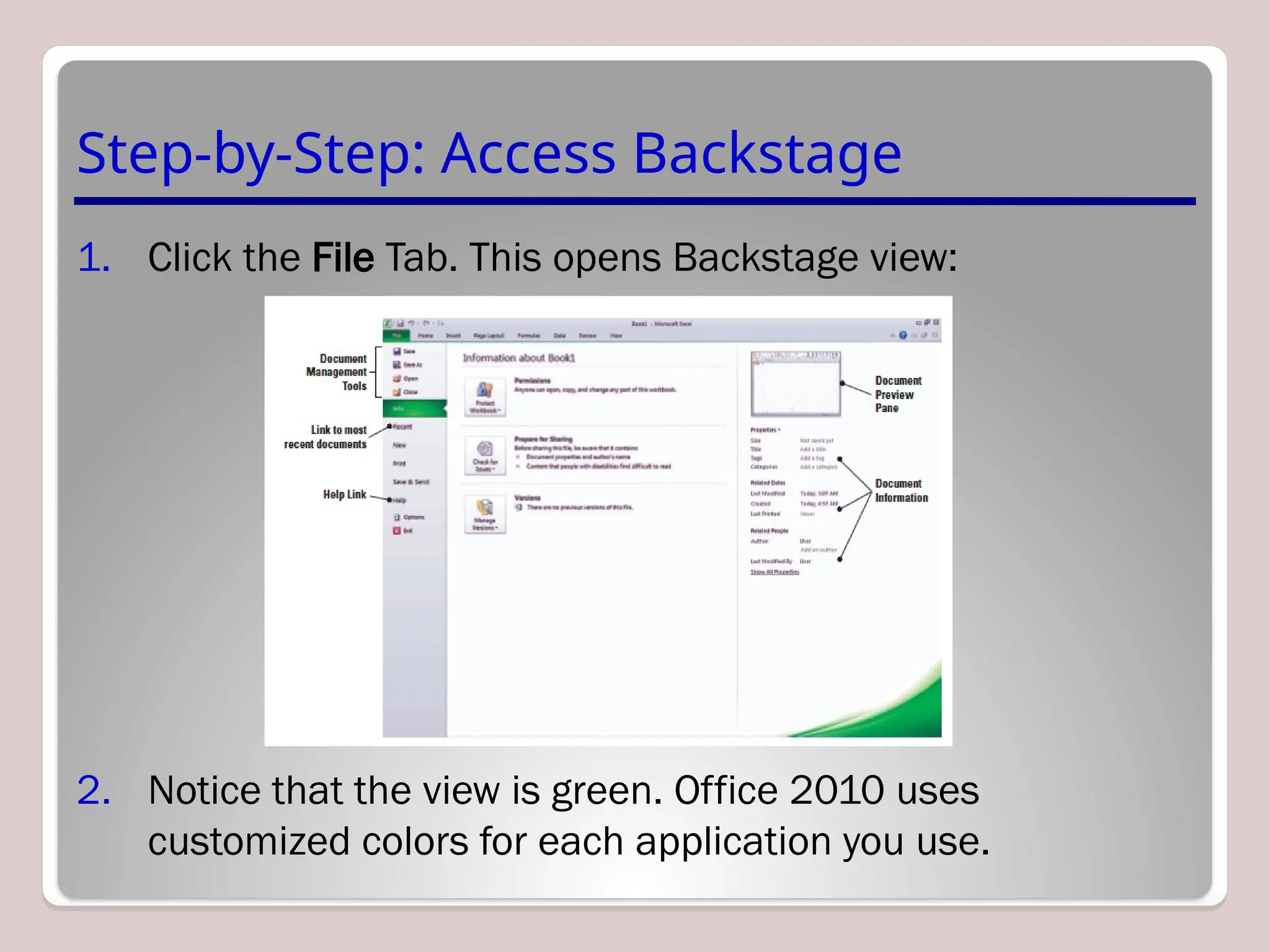
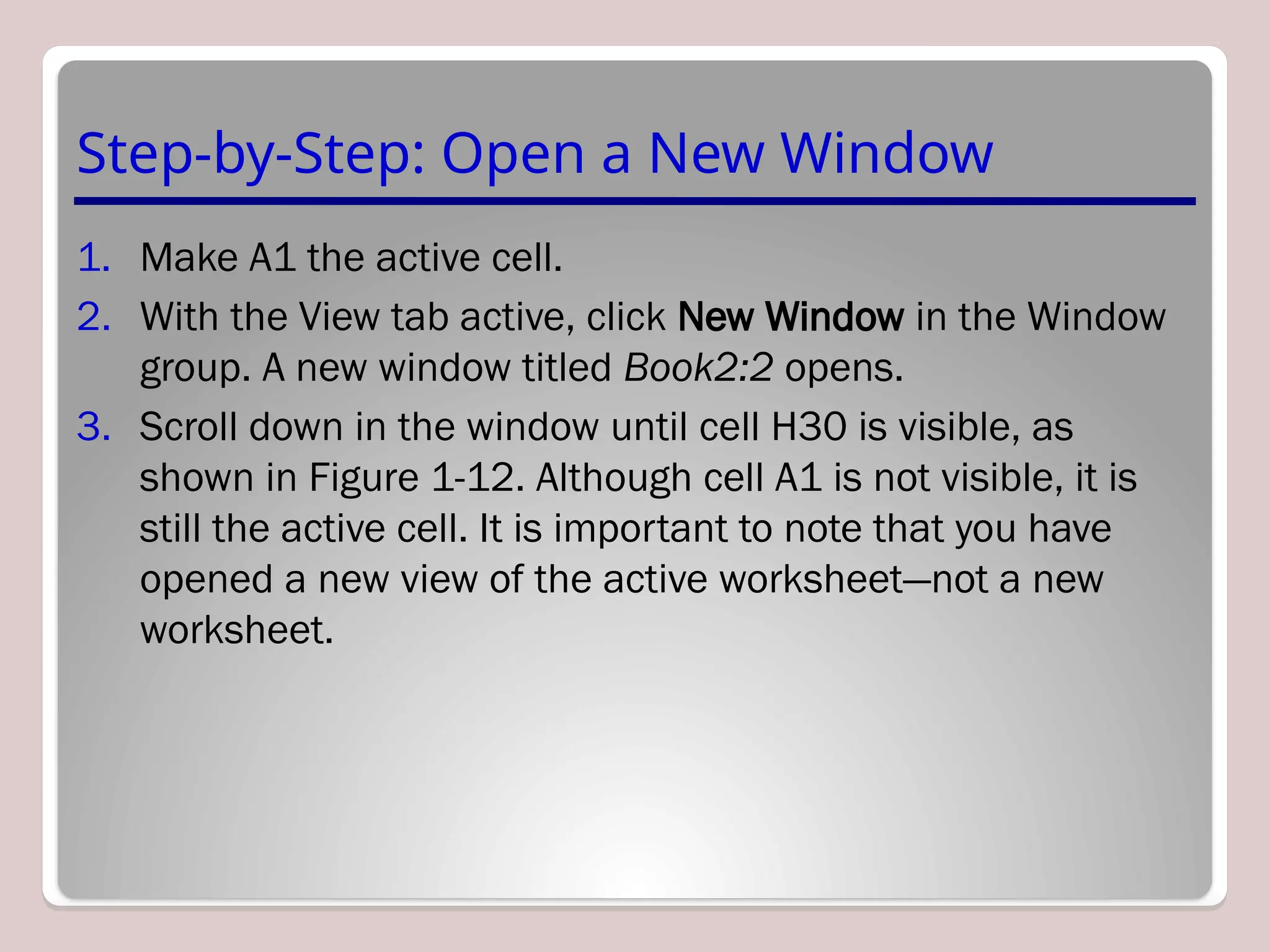
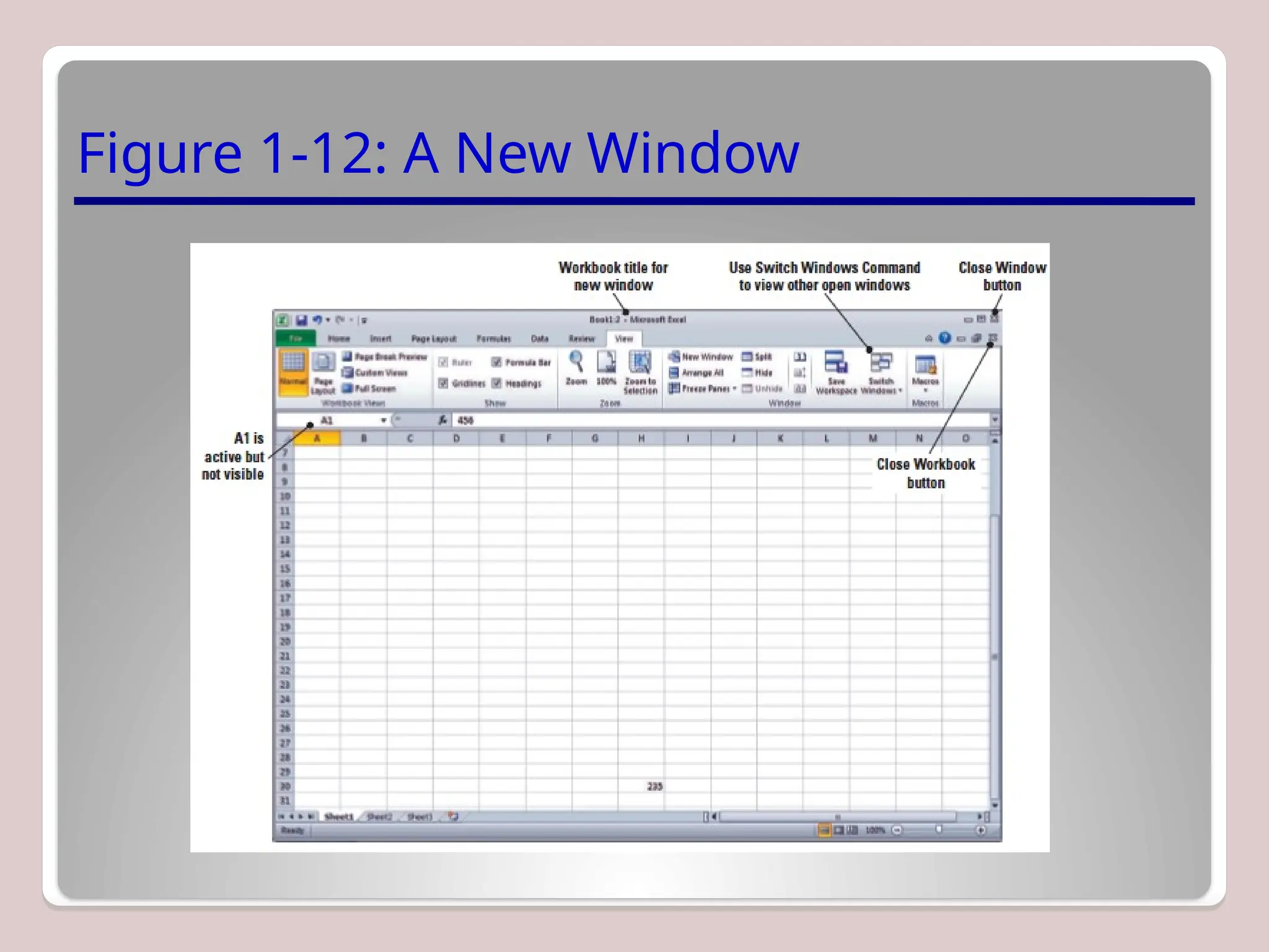
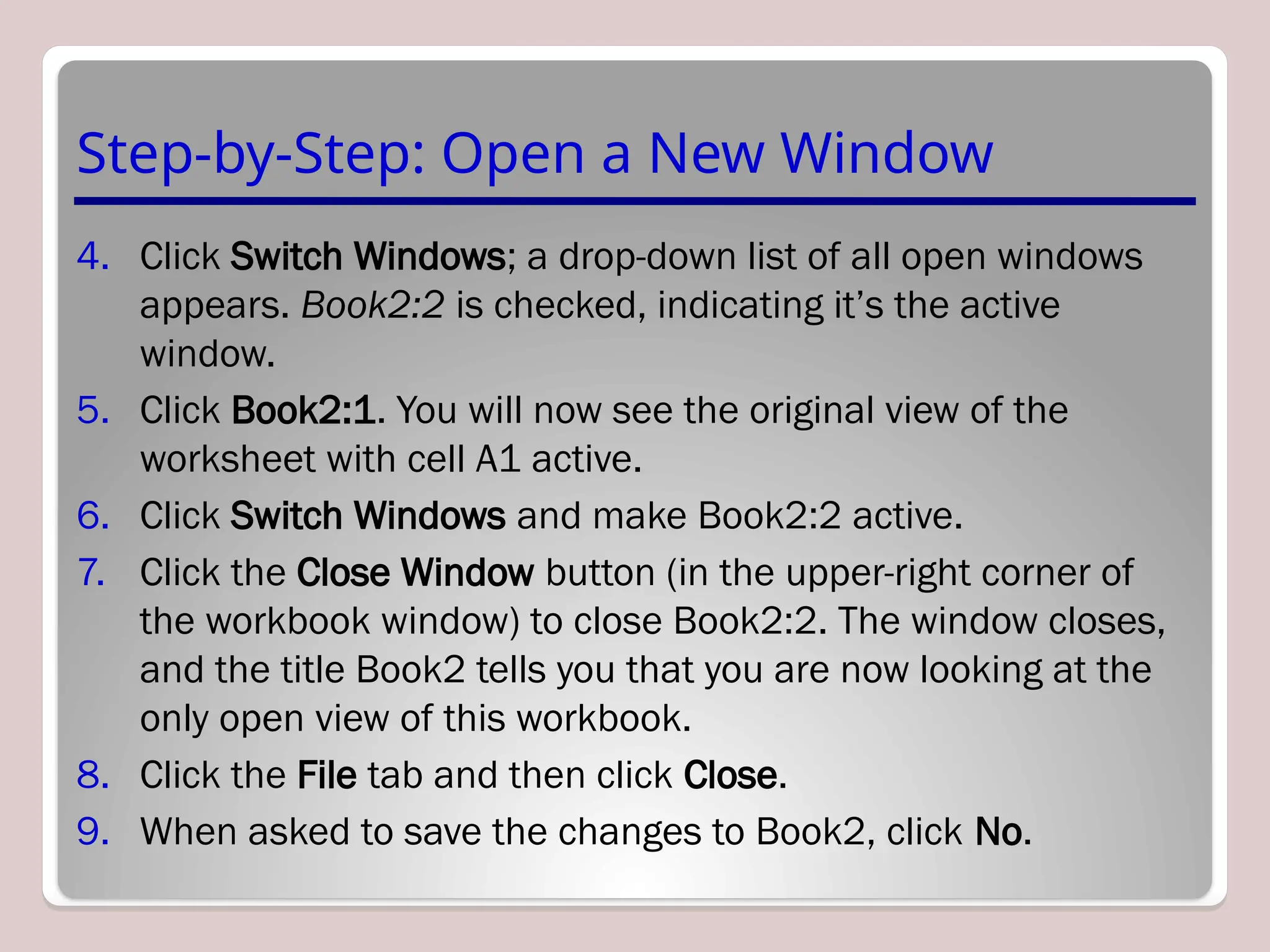
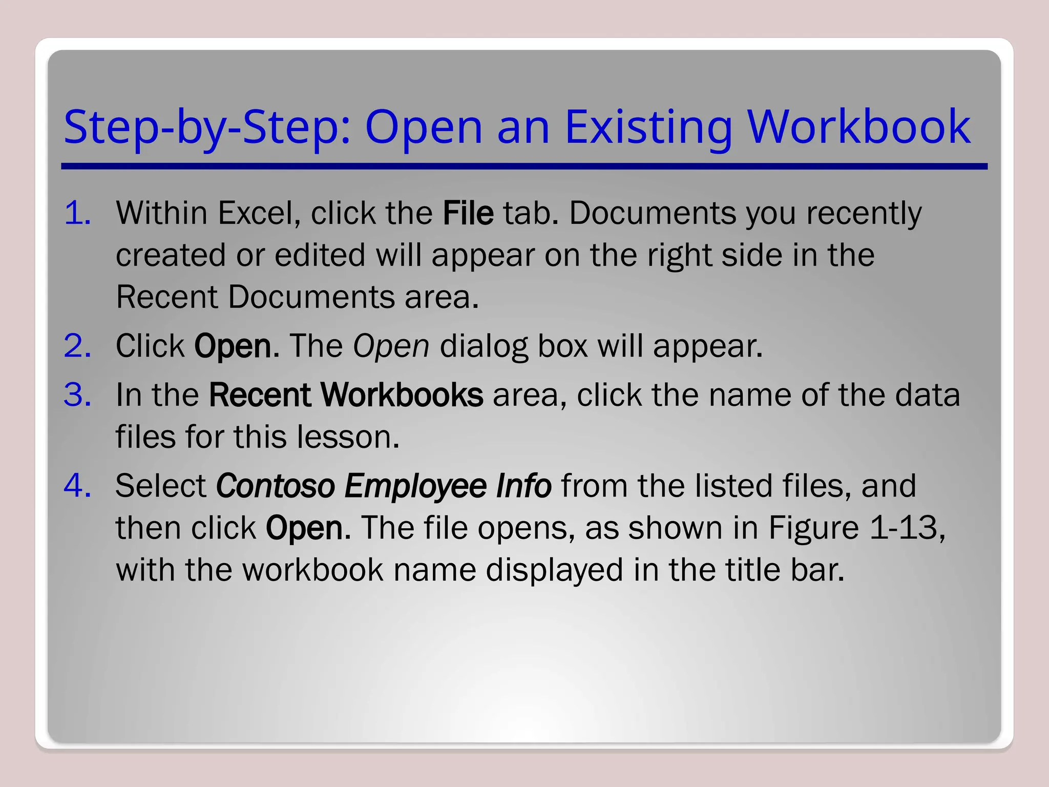
Overview
Lesson 1
Objectives
Step-by-Step: Start Excel
1. Click the Start menu, and then click All Programs.
2. On the list of programs, click Microsoft Office 2010.
3. Click Microsoft Office Excel 2010. A blank workbook will
open, and the worksheet named Sheet1 will be displayed.
Step-by-Step: Use Onscreen Tools
1. Place the cursor at the bottom of each command on the
Quick Access Toolbar and read the description that
appears as a ScreenTip.
2. Click the drop-down arrow at the right side of the Quick
Access Toolbar. From the drop-down list, select Open. The
Open icon is added to the Quick Access Toolbar. Click the
down arrow again and select Quick Print from the drop-
down list (see Figure 1-2).
Figure 1-2: Customizing the
Quick Access Toolbar
Step-by-Step: Use Onscreen Tools
3. Next, right-click the toolbar, then select Show Quick Access
Toolbar Below the Ribbon.
4. Right-click the Home tab and click Minimize the Ribbon;
now, only the tabs remain on display, increasing your
workspace.
5. Click the drop-down arrow on the right side of the Quick
Access Toolbar to produce a menu of options, then select
Minimize the Ribbon to turn off the option and make the
Ribbon commands visible.
Step-by-Step: Use Onscreen Tools
6. Right-click the Quick Access Toolbar again and choose
Show Quick Access Toolbar Above the Ribbon from the
pop-up menu.
7. Right-click the Open command, and select Remove from
Quick Access Toolbar.
NOTE: If you want to add commands to the Quick Access Toolbar
that don’t appear in the drop-down list, click More Commands on
the drop-down list. The Excel Options dialog box will open. You can
also right-click the Quick Access Toolbar or any Ribbon tab and
select Customize Quick Access Toolbar to open the Excel Options
window.
Step-by-Step: Navigate the Ribbon
1. With the Home tab active, click cell A1; your screen should
look similar to the one shown below.
Step-by-Step: Navigate the Ribbon
2. Click the Insert tab; your screen should now look similar to
the one shown below. Commands on the Insert tab enable
you to add charts and illustrations and to perform other
functions that enhance your Excel spreadsheets.
Step-by-Step: Navigate the Ribbon
3. Click the Home tab.
4. Press and release the Alt key to produce onscreen Keytips
that show keyboard shortcuts for certain commands (see
Figure 1-6).
5. Press the Esc key or press the Alt key again to turn off the
Keytips.
Step-by-Step: Access Backstage
1. Click the File Tab. This opens Backstage view:
2. Notice that the view is green. Office 2010 uses
customized colors for each application you use.
Step-by-Step: Use the File Tab to Open
Backstage View and Create a New
Workbook
1. Click the File tab to open Backstage view.
2. Click Close in the navigation bar; your workbook
disappears, but Excel remains open.
3. Click the File tab again, then click New; the Available
Templates pane opens (see the figure on the next slide).
Step-by-Step: Use the File Tab to Open
Backstage View and Create a New
Workbook
4. Click Blank Workbook in the Available Templates pane, and
then click Create. A new blank workbook is opened.
Step-by-Step: Change Excel’s View
1. The Home tab should be active. If not, click the Home tab.
2. Select cell A1 to make this cell active. Then type 456 and
press Tab.
3. Click the Dialog Box Launcher arrow in the lower-right
corner of the Font group of commands. The Format Cells
dialog box (shown below) opens.
Step-by-Step: Change Excel’s View
4. Notice that the Font tab of the dialog box is active. Change
the font to Arial, then click OK.
5. Cell B1 should now be the active cell in your worksheet.
Key 456 in this cell, then press Tab. Notice the difference
in size and appearance between this number and the one
you keyed in cell A1.
6. Click the View tab.
7. Click Page Layout view. Your workbook should look like
Figure 1-10 (shown on the next slide). In this view, you can
see the margins, and you can add a header or footer.
Figure 1-10: Page Layout View
Step-by-Step: Split a Window
1. Press Ctrl+Home to make cell A1 active.
2. With the View tab active, click the Split command in the
Window group.
3. Choose the lower-right quadrant by clicking any cell in that
area, then scroll down to Row 30.
4. Key 235 in cell H30 and press Enter. The data you entered
in cells A1 and B1 should be visible along with what you
just entered in cell H30, as shown in Figure 11-1 on the
next slide.
Step-by-Step: Split a Window
5. Click Split to remove the split. The data in cell H30 is no
longer visible. However, if you click the Split command once
more, you will again see all the data in this worksheet.
Step-by-Step: Open a New Window
1. Make A1 the active cell.
2. With the View tab active, click New Window in the Window
group. A new window titled Book2:2 opens.
3. Scroll down in the window until cell H30 is visible, as
shown in Figure 1-12. Although cell A1 is not visible, it is
still the active cell. It is important to note that you have
opened a new view of the active worksheet—not a new
worksheet.
Figure 1-12: A New Window
Step-by-Step: Open a New Window
4. Click Switch Windows; a drop-down list of all open windows
appears. Book2:2 is checked, indicating it’s the active
window.
5. Click Book2:1. You will now see the original view of the
worksheet with cell A1 active.
6. Click Switch Windows and make Book2:2 active.
7. Click the Close Window button (in the upper-right corner of
the workbook window) to close Book2:2. The window closes,
and the title Book2 tells you that you are now looking at the
only open view of this workbook.
8. Click the File tab and then click Close.
9. When asked to save the changes to Book2, click No.
Step-by-Step: Open an Existing Workbook
1. Within Excel, click the File tab. Documents you recently
created or edited will appear on the right side in the
Recent Documents area.
2. Click Open. The Open dialog box will appear.
3. In the Recent Workbooks area, click the name of the data
files for this lesson.
4. Select Contoso Employee Info from the listed files, and
then click Open. The file opens, as shown in Figure 1-13,
with the workbook name displayed in the title bar.
Figure 1-13: Opening an Existing
Worksheet
Step-by-Step: Navigate a Worksheet
1. Press Ctrl+Home to move to the beginning of the
document (cell A1).
2. Press Ctrl+End to move to the end of the document (cell
D27).
3. Click cell A27 to make it the active cell, and press Page Up.
The cursor moves to cell A1.
4. Click cell A3 to make it active, then press Ctrl+Page Down
to go to the last row of data (cell A27).
5. Press Ctrl+Right Arrow. The cursor moves to D27, the last
column in the range of data. The unused cells below the
data are considered a range.
Step-by-Step: Navigate a Worksheet
6. Press Ctrl+Down Arrow. The cursor moves to the last
possible row in the worksheet.
7. Press Ctrl+Home.
8. Press Scroll Lock while you press the Right Arrow key. This
moves the active column one column to the right.
9. Use the vertical scrollbar (refer to Figure 1-11) to navigate
from the beginning to the end of the data.
10.If your mouse has a wheel button, roll the wheel button
forward and back to quickly scroll through the worksheet.
NOTE: Ctrl+Arrow allows you to move to the start and end of
ranges of data. The title, which spans all the columns, is not
considered part of the worksheet’s data range.
Step-by-Step: Use the Help System
1. Position your mouse pointer over the Help button in the
upper-right corner of your Excel screen. A ScreenTip
appears, telling you that this button enables you to access
Excel’s Help features, as shown in the figure below.
Step-by-Step: Use the Help System
2. Click the Help button; the Help window opens, as shown in
the figure below.
Step-by-Step: Use the Help System
3. In the Help window, click on the Getting started with Excel
hyperlink. The next screen gives you additional hyperlinked
subcategories.
4. Navigate through 3 of the subtopics in the Help window.
5. Click the Office Help Connection Status button in the
bottom-right corner of the Help window. This displays the
Connection Status dialog box (shown below), which
enables you to choose whether the Help window displays
online or offline Help content.
Step-by-Step: Use the Help System
6. CLOSE the Help window.
Lesson Summary

Microsoft Excel introduction. Main functions

  • 1.
  • 2.
  • 3.
    Step-by-Step: Start Excel 1.Click the Start menu, and then click All Programs. 2. On the list of programs, click Microsoft Office 2010. 3. Click Microsoft Office Excel 2010. A blank workbook will open, and the worksheet named Sheet1 will be displayed.
  • 4.
    Step-by-Step: Use OnscreenTools 1. Place the cursor at the bottom of each command on the Quick Access Toolbar and read the description that appears as a ScreenTip. 2. Click the drop-down arrow at the right side of the Quick Access Toolbar. From the drop-down list, select Open. The Open icon is added to the Quick Access Toolbar. Click the down arrow again and select Quick Print from the drop- down list (see Figure 1-2).
  • 5.
    Figure 1-2: Customizingthe Quick Access Toolbar
  • 6.
    Step-by-Step: Use OnscreenTools 3. Next, right-click the toolbar, then select Show Quick Access Toolbar Below the Ribbon. 4. Right-click the Home tab and click Minimize the Ribbon; now, only the tabs remain on display, increasing your workspace. 5. Click the drop-down arrow on the right side of the Quick Access Toolbar to produce a menu of options, then select Minimize the Ribbon to turn off the option and make the Ribbon commands visible.
  • 7.
    Step-by-Step: Use OnscreenTools 6. Right-click the Quick Access Toolbar again and choose Show Quick Access Toolbar Above the Ribbon from the pop-up menu. 7. Right-click the Open command, and select Remove from Quick Access Toolbar. NOTE: If you want to add commands to the Quick Access Toolbar that don’t appear in the drop-down list, click More Commands on the drop-down list. The Excel Options dialog box will open. You can also right-click the Quick Access Toolbar or any Ribbon tab and select Customize Quick Access Toolbar to open the Excel Options window.
  • 8.
    Step-by-Step: Navigate theRibbon 1. With the Home tab active, click cell A1; your screen should look similar to the one shown below.
  • 9.
    Step-by-Step: Navigate theRibbon 2. Click the Insert tab; your screen should now look similar to the one shown below. Commands on the Insert tab enable you to add charts and illustrations and to perform other functions that enhance your Excel spreadsheets.
  • 10.
    Step-by-Step: Navigate theRibbon 3. Click the Home tab. 4. Press and release the Alt key to produce onscreen Keytips that show keyboard shortcuts for certain commands (see Figure 1-6). 5. Press the Esc key or press the Alt key again to turn off the Keytips.
  • 11.
    Step-by-Step: Access Backstage 1.Click the File Tab. This opens Backstage view: 2. Notice that the view is green. Office 2010 uses customized colors for each application you use.
  • 12.
    Step-by-Step: Use theFile Tab to Open Backstage View and Create a New Workbook 1. Click the File tab to open Backstage view. 2. Click Close in the navigation bar; your workbook disappears, but Excel remains open. 3. Click the File tab again, then click New; the Available Templates pane opens (see the figure on the next slide).
  • 13.
    Step-by-Step: Use theFile Tab to Open Backstage View and Create a New Workbook 4. Click Blank Workbook in the Available Templates pane, and then click Create. A new blank workbook is opened.
  • 14.
    Step-by-Step: Change Excel’sView 1. The Home tab should be active. If not, click the Home tab. 2. Select cell A1 to make this cell active. Then type 456 and press Tab. 3. Click the Dialog Box Launcher arrow in the lower-right corner of the Font group of commands. The Format Cells dialog box (shown below) opens.
  • 15.
    Step-by-Step: Change Excel’sView 4. Notice that the Font tab of the dialog box is active. Change the font to Arial, then click OK. 5. Cell B1 should now be the active cell in your worksheet. Key 456 in this cell, then press Tab. Notice the difference in size and appearance between this number and the one you keyed in cell A1. 6. Click the View tab. 7. Click Page Layout view. Your workbook should look like Figure 1-10 (shown on the next slide). In this view, you can see the margins, and you can add a header or footer.
  • 16.
    Figure 1-10: PageLayout View
  • 17.
    Step-by-Step: Split aWindow 1. Press Ctrl+Home to make cell A1 active. 2. With the View tab active, click the Split command in the Window group. 3. Choose the lower-right quadrant by clicking any cell in that area, then scroll down to Row 30. 4. Key 235 in cell H30 and press Enter. The data you entered in cells A1 and B1 should be visible along with what you just entered in cell H30, as shown in Figure 11-1 on the next slide.
  • 18.
    Step-by-Step: Split aWindow 5. Click Split to remove the split. The data in cell H30 is no longer visible. However, if you click the Split command once more, you will again see all the data in this worksheet.
  • 19.
    Step-by-Step: Open aNew Window 1. Make A1 the active cell. 2. With the View tab active, click New Window in the Window group. A new window titled Book2:2 opens. 3. Scroll down in the window until cell H30 is visible, as shown in Figure 1-12. Although cell A1 is not visible, it is still the active cell. It is important to note that you have opened a new view of the active worksheet—not a new worksheet.
  • 20.
    Figure 1-12: ANew Window
  • 21.
    Step-by-Step: Open aNew Window 4. Click Switch Windows; a drop-down list of all open windows appears. Book2:2 is checked, indicating it’s the active window. 5. Click Book2:1. You will now see the original view of the worksheet with cell A1 active. 6. Click Switch Windows and make Book2:2 active. 7. Click the Close Window button (in the upper-right corner of the workbook window) to close Book2:2. The window closes, and the title Book2 tells you that you are now looking at the only open view of this workbook. 8. Click the File tab and then click Close. 9. When asked to save the changes to Book2, click No.
  • 22.
    Step-by-Step: Open anExisting Workbook 1. Within Excel, click the File tab. Documents you recently created or edited will appear on the right side in the Recent Documents area. 2. Click Open. The Open dialog box will appear. 3. In the Recent Workbooks area, click the name of the data files for this lesson. 4. Select Contoso Employee Info from the listed files, and then click Open. The file opens, as shown in Figure 1-13, with the workbook name displayed in the title bar.
  • 23.
    Figure 1-13: Openingan Existing Worksheet
  • 24.
    Step-by-Step: Navigate aWorksheet 1. Press Ctrl+Home to move to the beginning of the document (cell A1). 2. Press Ctrl+End to move to the end of the document (cell D27). 3. Click cell A27 to make it the active cell, and press Page Up. The cursor moves to cell A1. 4. Click cell A3 to make it active, then press Ctrl+Page Down to go to the last row of data (cell A27). 5. Press Ctrl+Right Arrow. The cursor moves to D27, the last column in the range of data. The unused cells below the data are considered a range.
  • 25.
    Step-by-Step: Navigate aWorksheet 6. Press Ctrl+Down Arrow. The cursor moves to the last possible row in the worksheet. 7. Press Ctrl+Home. 8. Press Scroll Lock while you press the Right Arrow key. This moves the active column one column to the right. 9. Use the vertical scrollbar (refer to Figure 1-11) to navigate from the beginning to the end of the data. 10.If your mouse has a wheel button, roll the wheel button forward and back to quickly scroll through the worksheet. NOTE: Ctrl+Arrow allows you to move to the start and end of ranges of data. The title, which spans all the columns, is not considered part of the worksheet’s data range.
  • 26.
    Step-by-Step: Use theHelp System 1. Position your mouse pointer over the Help button in the upper-right corner of your Excel screen. A ScreenTip appears, telling you that this button enables you to access Excel’s Help features, as shown in the figure below.
  • 27.
    Step-by-Step: Use theHelp System 2. Click the Help button; the Help window opens, as shown in the figure below.
  • 28.
    Step-by-Step: Use theHelp System 3. In the Help window, click on the Getting started with Excel hyperlink. The next screen gives you additional hyperlinked subcategories. 4. Navigate through 3 of the subtopics in the Help window. 5. Click the Office Help Connection Status button in the bottom-right corner of the Help window. This displays the Connection Status dialog box (shown below), which enables you to choose whether the Help window displays online or offline Help content.
  • 29.
    Step-by-Step: Use theHelp System 6. CLOSE the Help window.
  • 30.

Editor's Notes

  • #5 If you want to add a command to the Quick Access Toolbar, you can also right-click any icon on the Ribbon and then click Add to Quick Access Toolbar.
  • #10 Keyboard shortcuts enable you to issue commands in Excel without using the mouse (so you don’t have to take your hands from the keyboard). Keyboard shortcuts are used by pressing the key shown in the Keytip while also pressing and holding the Alt key. When you press and release the Alt key by itself, Excel displays the shortcuts for the Quick Access Toolbar.
  • #11 The use and tools of Backstage are covered in depth in Lesson 2.
  • #15 Another way to change a font is by typing the first few letters of the name of the font you’re searching for; Excel will locate it on the font list. You can also scroll through the list and choose your font type.
  • #18 The Split command is especially useful when you need to compare various portions of a long worksheet.
  • #21 Step 7 Note: Clicking the Close Window button will close only the new window opened at the beginning of this exercise. If you use the Close command in the Microsoft File tab, you will close the entire workbook.
  • #22 Step 2 Note: By default, the Open dialog box lists only the files that were created in the program you are using—in this case, Excel. To see files created in other programs, you can select All Files in the Files of type box at the bottom of the Open dialog box.
  • #25 If you’d like to refer to Figure 11-1, it’s shown in Slide 28. Step 8 Note: When Scroll Lock is on, scroll lock is displayed on the left side of the Status bar. If you want to use the arrow keys to move between cells, you must turn off Scroll Lock. Some keyboards come equipped with an onboard scroll lock key, while others do not. This is an option not a necessity.
  • #28 Step 5 Note: Even if Excel is set to work offline, you can still search for help online. To do so, instead of clicking the Search button, click the drop-down arrow next to it. When the menu appears, click the Content from Office Online link. The choice will affect only the current search, not Excel’s overall settings.