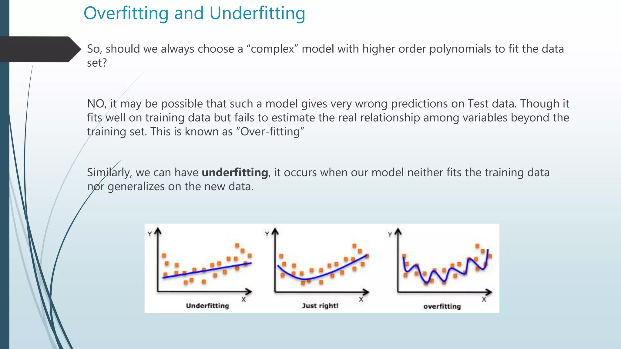
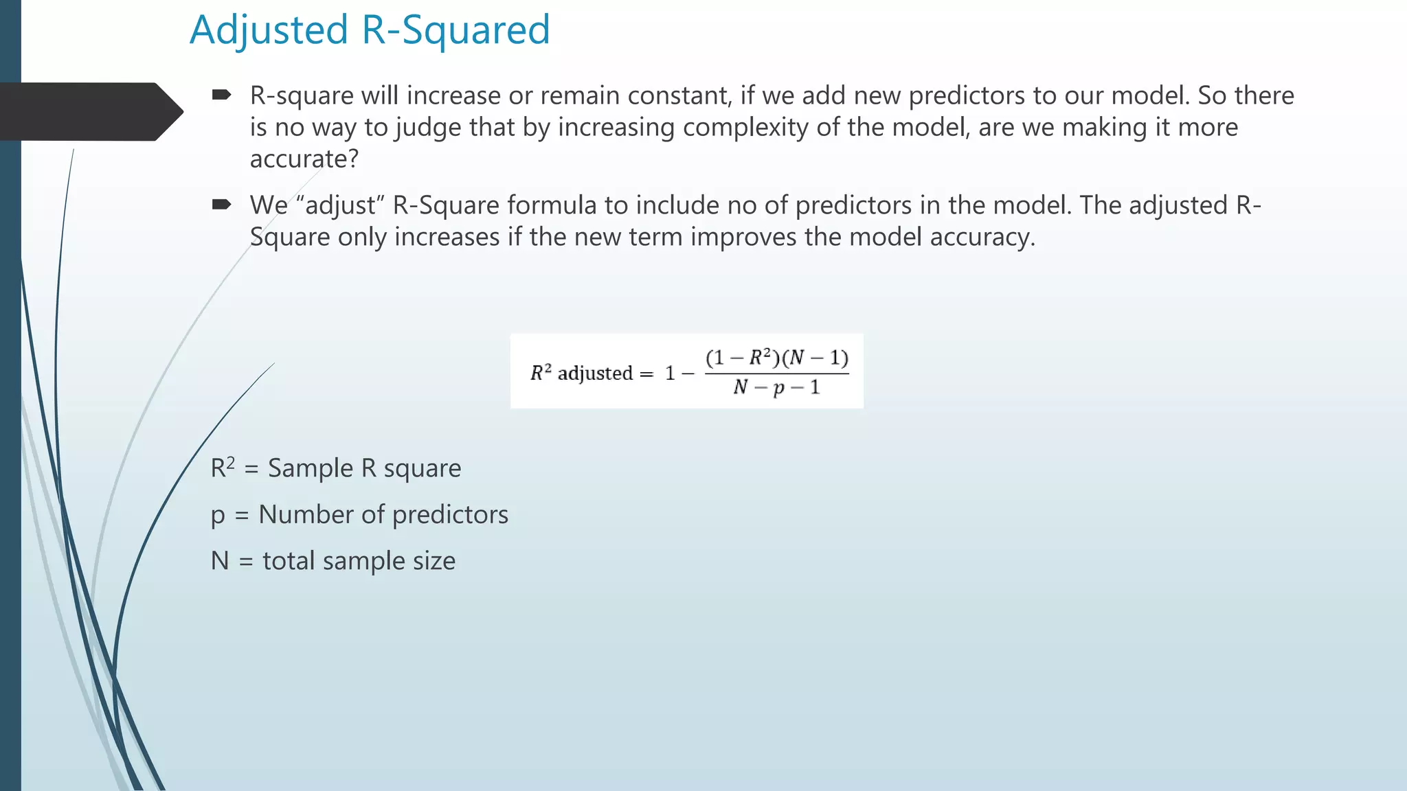
Machine learning session4(linear regression)

Linear Regression
 Linear regression: Linear regression involves using data to calculate a line that best
fits that data, and then using that line to predict scores on one variable from another.
Prediction is simply the process of estimating scores of the outcome (or dependent)
variable based on the scores of the predictor (or independent) variable. To generate
the regression line, we look for a line of best fit. A line which can explain the
relationship between independent and dependent variable(s), better is said to be best
fit line. The difference between the observed value and actual value gives the error.
Linear Regression gives an equation of the following form:
Y = m0 + m1x1 + m2x2 + m3x3 +…….mnxn
where Y is the dependent variable and X’s are the independent variables.
The right-hand side of this equation is also known as Hypothesis Function - H(x)

Line of Best Fit
The purpose of line of best fit is that the predicted values
should be as close as possible to the actual or observed
values. This means the main objective in determining the line
of best fit is to “minimize” the difference predicted values and
observed values. These differences are called “errors” or
“residuals”.
3 ways to calculate the “error”
 Sum of all errors: (∑(Y – h(X))) (This may result in
the cancellation of positive and negative errors.
This will not be a correct metric to use)
 Sum of absolute value of all errors: (∑|Y-h(X)|)
 Sum of square of all errors ( ∑ (Y-h(X))2)
 The line of best fit for 1 feature can be represented as :
Y= bx +c Where Y is the score or outcome
variable we are trying to predict
B = regression coefficient or slope
C = Y intercept or the regression constant
This is Linear regression with 1 variable.

Sum of Squared Errors
 Squaring the difference between actual value and predicted value “penalizes” more for
each error. Hence minimizing the sum of squared errors improves the quality of regression
line.
 This method of fitting the data line so that there is minimal difference between the
observations and the line is called the method of least squares.
 Baseline model refers to the line which predicts each value as the average of the data
points.
 SSE or Sum of Squared Errors is the total of all squares of the errors. It is a measure of
the quality of regression line. SSE is sensitive to the number of input data points.
 SST is Total Sum of Squares: It is the SSE for baseline model.

Regression Metrics
Mean Absolute Error : One way to measure error is by using absolute error to find the predicted
distance from the true value. The mean absolute error takes the total absolute error of each example
and averages the error based on the number of data points. By adding up all the absolute values of
errors of a model we can avoid canceling out errors from being too high or below the true values and
get an overall error metric to evaluate the model on.
Mean Squared Error : Mean squared is the most common metric to measure model performance. In
contrast with absolute error, the residual error (the difference between predicted and the true value)
is squared.
Some benefits of squaring the residual error is that error terms are positive, it emphasizes larger
errors over smaller errors, and is differentiable. Being differentiable allows us to use calculus to find
minimum or maximum values, often resulting in being more computationally efficient.
R-Squared: Its called coefficient of determination. The values for R2 range from 0 to 1, and it
determines how much of the total variation in Y is explained by the variation in X. A model with an
R2 of 0 is no better than a model that always predicts the mean of the target variable, whereas a
model with an R2 of 1 perfectly predicts the target variable. Any value between 0 and 1 indicates what
percentage of the target variable, using this model, can be explained by the features. A model can be
given a negative R2 as well, which indicates that the model is arbitrarily worse than one that always
predicts the mean of the target variable.

Cost Function
 The error of regression model is expressed as a cost function :
Its is similar to sum of squared errors. 1/m is means, we are calculating the average. The factor
½ is used to simplify mathematics. This function is minimized to reduce errors in prediction.
Minimizing this function, means we get the values of θ0 and θ1 which find on average the
minimal deviation of x from y when we use those parameters in our hypothesis function.

Inside Cost Function
Cost function :
Lets assume, θ0 is 0. (Our hypothesis passes through origin)
So, now we need that value of θ1 for which Cost function is minimum. To find that out, plot
J(θ1) vs θ1

Inside Cost Function
Cost function :
With both θ0 and θ1, The plot becomes more complex
So, now we need that value of θ1 for which Cost function is minimum. To find that out, plot
J(θ1, θ0 ) vs θ1 and θ0

Gradient Descent
The process of minimizing the cost function can be
achieved by Gradient Descent algorithm:
The steps are:
1. Start with initial guess of coefficients
2. Keep changing the coefficients a little bit to try
and reduce Cost Function J(θ0,θ1)
3. Each time, the parameters are changed, the
gradient is chosen which reduces J(θ0,θ1) the
most.
4. Repeat
5. Keep doing till no improvement is made.

Polynomial Regression
Instead of finding a best fit “line” on the given data
points, we can also try to find the best fit “curve”.
This is the form of Polynomial regression. The equation,
in case of second-order polynomial will be:
Y = θ0+ θ1x+ θ2x2 (Quadratic Regression)
Third-order polynomial will be:
Y = θ0+ θ1x+ θ2x2 + θ3x3 (Cubic Regression)
When we use higher order powers in our regression
model, we say that we are increasing the “complexity”
of the model. The more the complexity of the model,
the better it will “fit” on the given data.

Overfitting and Underfitting
So, should we always choose a “complex” model with higher order polynomials to fit the data
set?
NO, it may be possible that such a model gives very wrong predictions on Test data. Though it
fits well on training data but fails to estimate the real relationship among variables beyond the
training set. This is known as “Over-fitting”
Similarly, we can have underfitting, it occurs when our model neither fits the training data
nor generalizes on the new data.

Bias and Variance
Bias: Bias occurs when a model has enough data but is not complex enough to capture the
underlying relationships(or patterns). As a result, the model consistently and systematically
misrepresents the data, leading to low accuracy in prediction. This is known as underfitting.
Simply put, bias occurs when we have an inadequate model. (Pays too little attention to data;
does the same thing over and over again; high error on training set)
Variance: When training a model, we typically use a limited number of samples from a larger
population. If we repeatedly train a model with randomly selected subsets of data, we would
expect its predictions to be different based on the specific examples given to it.
Here variance is a measure of how much the predictions vary for any given test sample. (Pays
too much attention to data; high error on test set)
 Some variance is normal, but too much variance indicates that the model is unable to
generalize its predictions to the larger population. High sensitivity to the training set is
also known as overfitting, and generally occurs when either the model is too complex or
when we do not have enough data to support it.
 We can typically reduce the variability of a model's predictions and increase precision by
training on more data. If more data is unavailable, we can also control variance by limiting
our model's complexity.

Adjusted R-Squared
 R-square will increase or remain constant, if we add new predictors to our model. So there
is no way to judge that by increasing complexity of the model, are we making it more
accurate?
 We “adjust” R-Square formula to include no of predictors in the model. The adjusted R-
Square only increases if the new term improves the model accuracy.
R2 = Sample R square
p = Number of predictors
N = total sample size

Machine learning session4(linear regression)

More Related Content

What's hot

Similar to Machine learning session4(linear regression)

More from Abhimanyu Dwivedi

Recently uploaded

Machine learning session4(linear regression)