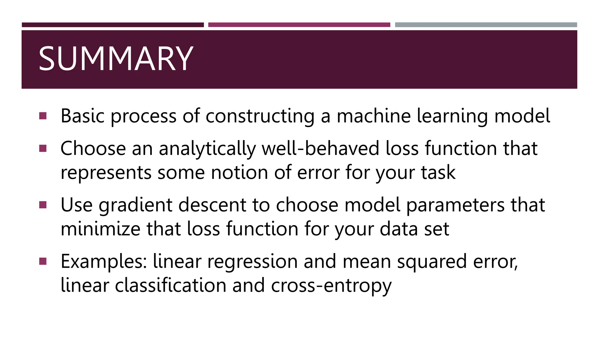
This document provides an introduction to machine learning concepts including linear regression, linear classification, and the cross-entropy loss function. It discusses using gradient descent to fit machine learning models by minimizing a loss function on training data. Specifically, it describes how linear regression can be solved using mean squared error and gradient descent, and how linear classifiers can be trained with the cross-entropy loss and softmax activations. The goal is to choose model parameters that minimize the loss function for a given dataset.


![PROBABILISTIC INTERPRETATION
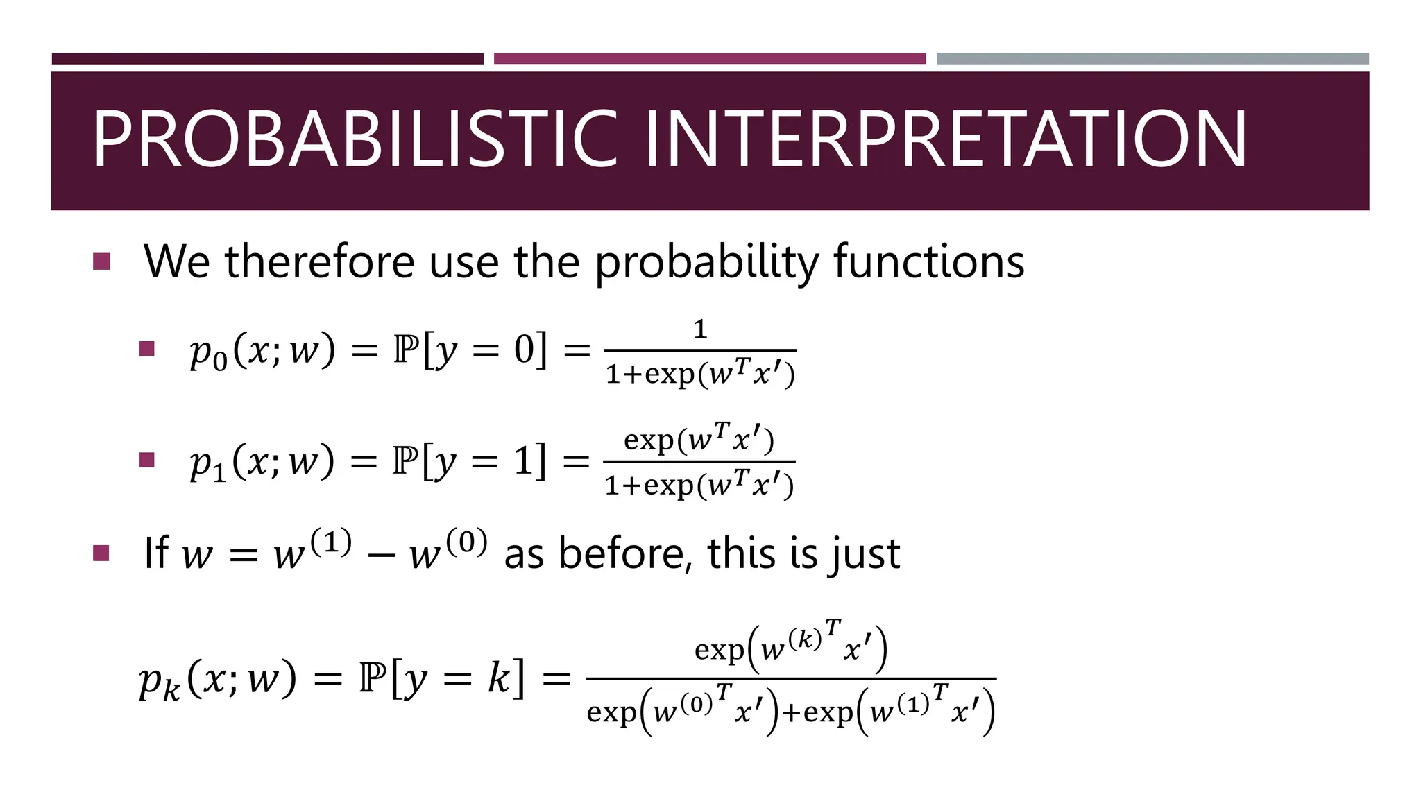
Interpreting 𝑤𝑇
𝑥′
𝑤𝑇
𝑥′ large and positive
ℙ 𝑦 = 0 ≪ ℙ[𝑦 = 1]
𝑤𝑇
𝑥′ large and negative
ℙ 𝑦 = 0 ≫ ℙ[𝑦 = 1]
𝑤𝑇
𝑥′ small
ℙ 𝑦 = 0 ≈ ℙ[𝑦 = 1]](https://image.slidesharecdn.com/cs1792019lec13-240416180809-2cc457e5/75/Machine-learning-introduction-lecture-notes-31-2048.jpg)


![Coded Agents – with UiPath SDK + LangGraph [Virtual Hands-on Workshop]](https://cdn.slidesharecdn.com/ss_thumbnails/codedagentsdeck-251215155422-5497c599-thumbnail.jpg?width=640&height=640&fit=bounds)


