THE CRUX: HOWTO DEVELOP SCHEDULING POLICY
How should we develop a basic framework for thinking about
scheduling policies?
What are the key assumptions?
What metrics are important?
What basic approaches have been used in the earliest of computer
systems?
4.
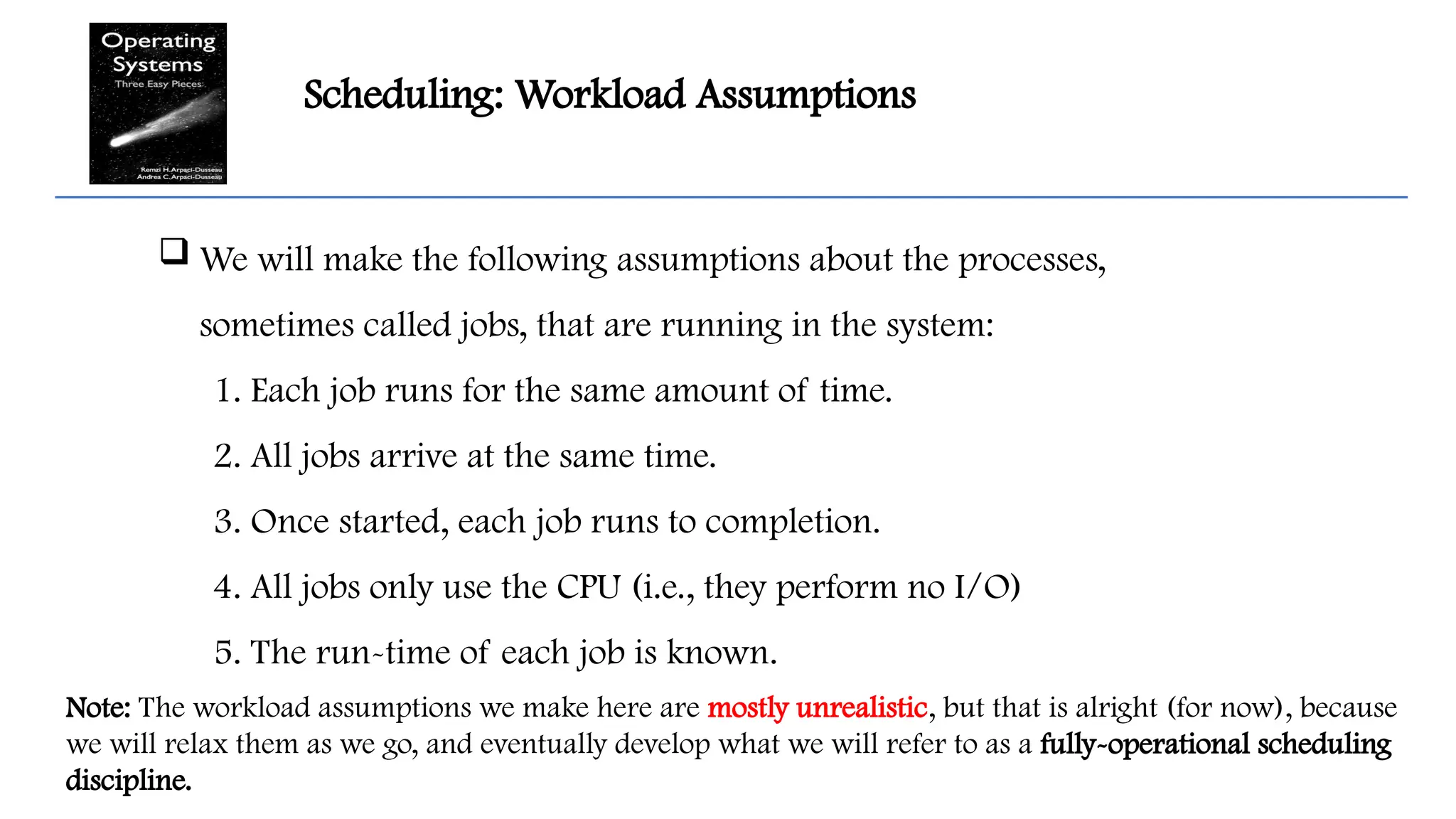
Scheduling: Workload Assumptions
We will make the following assumptions about the processes,
sometimes called jobs, that are running in the system:
1. Each job runs for the same amount of time.
2. All jobs arrive at the same time.
3. Once started, each job runs to completion.
4. All jobs only use the CPU (i.e., they perform no I/O)
5. The run-time of each job is known.
Note: The workload assumptions we make here are mostly unrealistic, but that is alright (for now), because
we will relax them as we go, and eventually develop what we will refer to as a fully-operational scheduling
discipline.
5.
Scheduling: Scheduling Metrics
To enable us to compare different scheduling policies, we need a
scheduling metric.
Turnaround Time(Performance metric): The time at which the job
completes minus the time at which the job arrived at the system.
Tturnaround = Tcompletion T
− arrival
Fairness
Performance and fairness are often at odds.
6.
Scheduling: First In,First Out (FIFO)
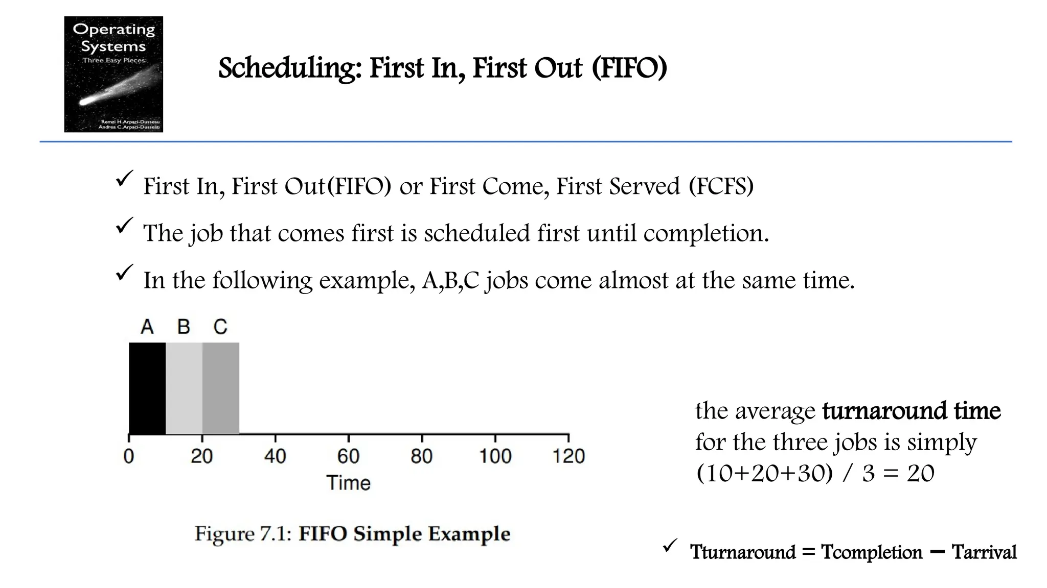
First In, First Out(FIFO) or First Come, First Served (FCFS)
The job that comes first is scheduled first until completion.
In the following example, A,B,C jobs come almost at the same time.
the average turnaround time
for the three jobs is simply
(10+20+30) / 3 = 20
Tturnaround = Tcompletion T
− arrival
7.
Scheduling: First In,First Out (FIFO)
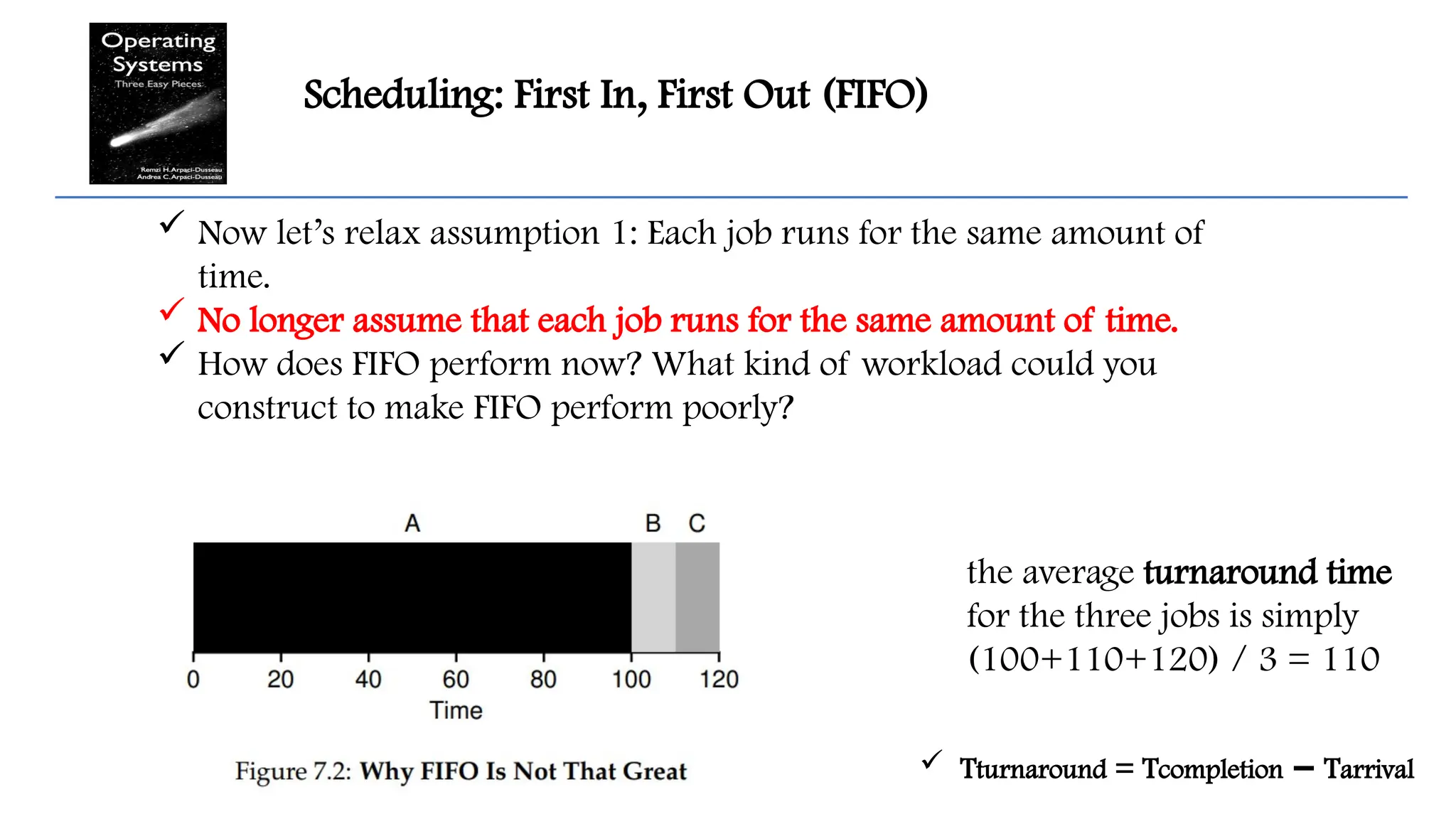
Now let’s relax assumption 1: Each job runs for the same amount of
time.
No longer assume that each job runs for the same amount of time.
How does FIFO perform now? What kind of workload could you
construct to make FIFO perform poorly?
the average turnaround time
for the three jobs is simply
(100+110+120) / 3 = 110
Tturnaround = Tcompletion T
− arrival
8.
Scheduling: First In,First Out (FIFO)
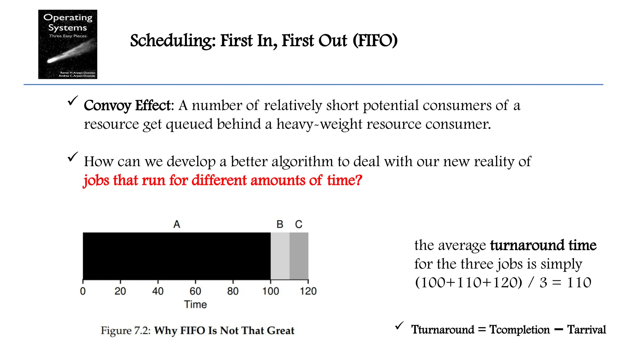
Convoy Effect: A number of relatively short potential consumers of a
resource get queued behind a heavy-weight resource consumer.
How can we develop a better algorithm to deal with our new reality of
jobs that run for different amounts of time?
the average turnaround time
for the three jobs is simply
(100+110+120) / 3 = 110
Tturnaround = Tcompletion T
− arrival
9.
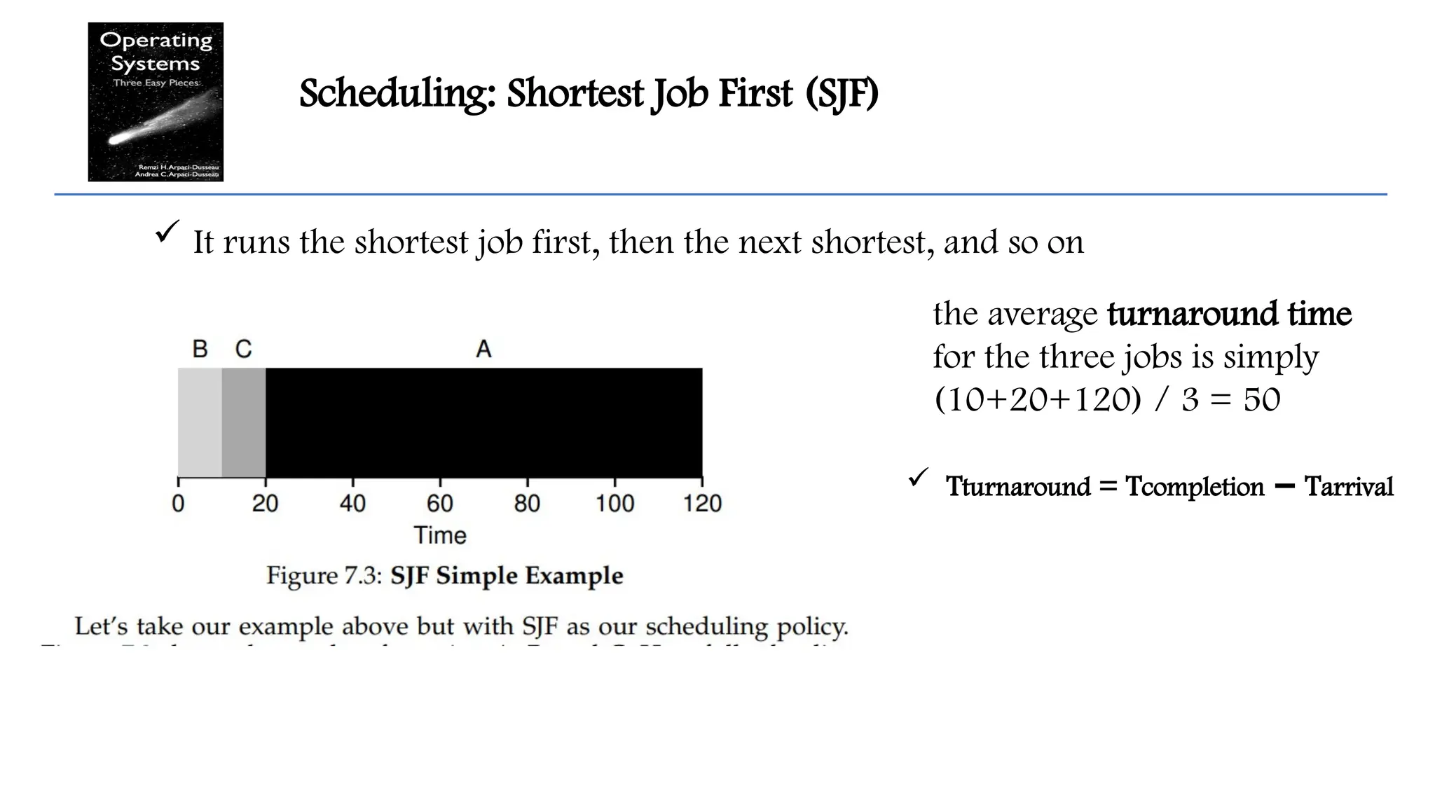
Scheduling: Shortest JobFirst (SJF)
It runs the shortest job first, then the next shortest, and so on
the average turnaround time
for the three jobs is simply
(10+20+120) / 3 = 50
Tturnaround = Tcompletion T
− arrival
10.
Scheduling: Shortest JobFirst (SJF)
Given our assumptions about jobs all arriving at the same time, we
could prove that SJF is indeed an optimal scheduling algorithm.
However, you are in a systems class, not theory or operations research;
no proofs are allowed.
Let’s relax our assumption 2: All jobs arrive at the same time.
Now assume that jobs can arrive at any time instead of all at once.
11.
Scheduling: Shortest JobFirst (SJF)
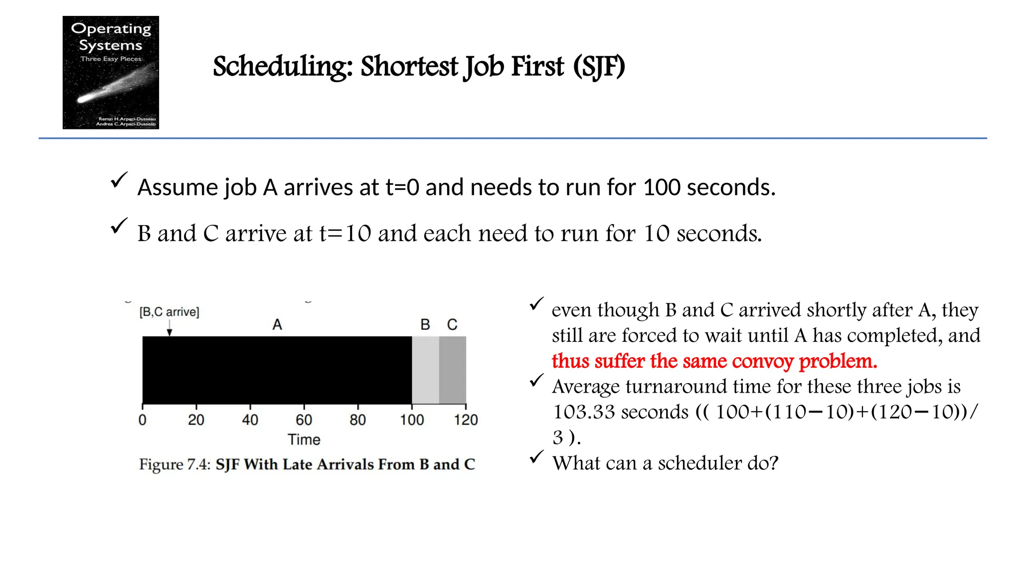
Assume job A arrives at t=0 and needs to run for 100 seconds.
B and C arrive at t=10 and each need to run for 10 seconds.
even though B and C arrived shortly after A, they
still are forced to wait until A has completed, and
thus suffer the same convoy problem.
Average turnaround time for these three jobs is
103.33 seconds (( 100+(110 10)+(120 10))/
− −
3 ).
What can a scheduler do?
12.
Scheduling: Shortest Time-to-CompletionFirst (STCF)
To address this concern, we need to relax assumption 3: Once started,
each job runs to completion.
We can interrupt a job while it is executing – known as preemption.
The scheduler should be able to preempt a job, and decide to run
another job.
Any time a new job enters the system, the STCF scheduler determines
which of the remaining jobs (including the new job) has the least time
left, and schedules that one.
13.
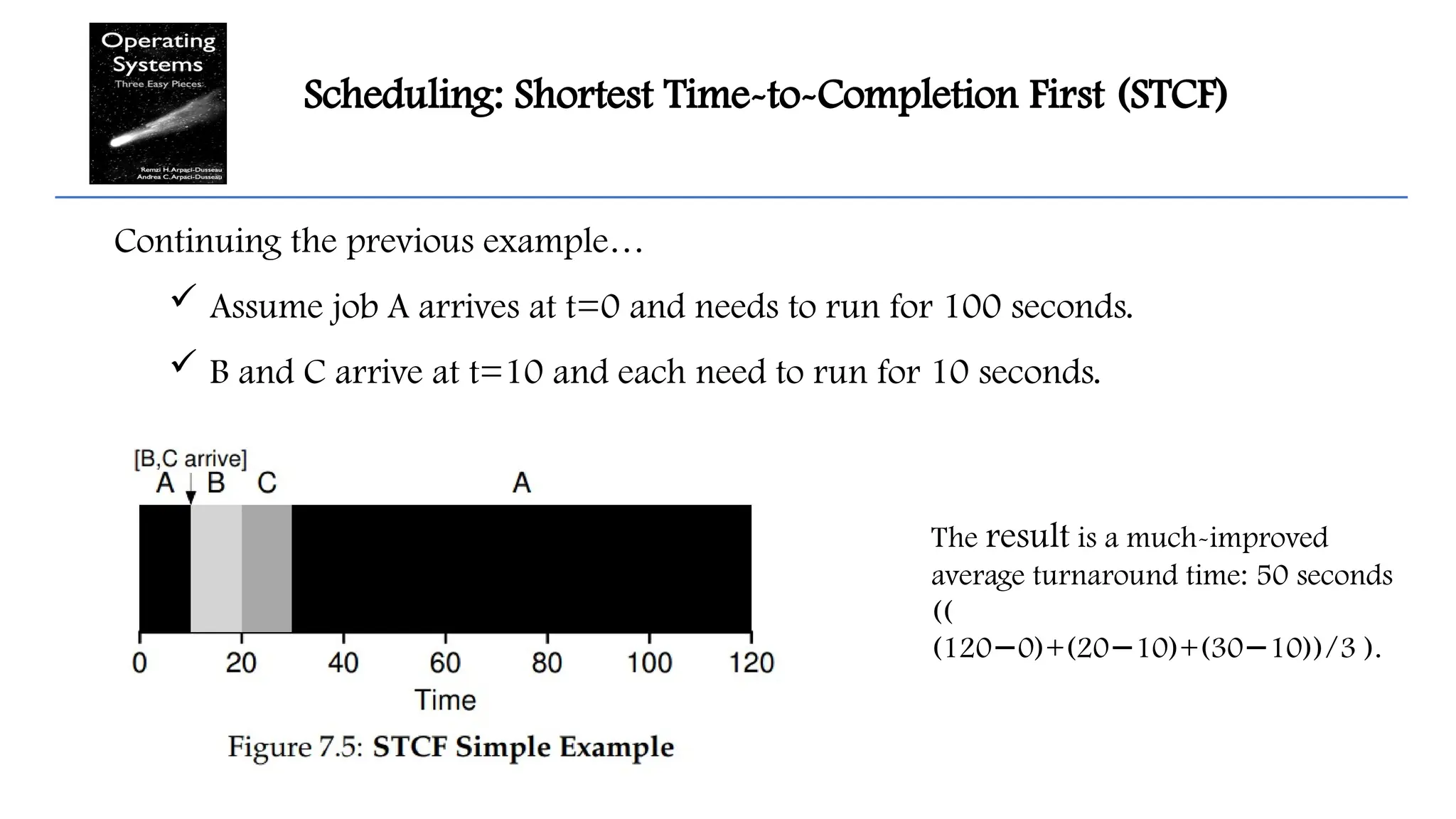
Scheduling: Shortest Time-to-CompletionFirst (STCF)
The result is a much-improved
average turnaround time: 50 seconds
((
(120 0)+(20 10)+(30 10))/3 ).
− − −
Continuing the previous example…
Assume job A arrives at t=0 and needs to run for 100 seconds.
B and C arrive at t=10 and each need to run for 10 seconds.
14.
Scheduling: A NewMetric – Response Time
A New Scheduling – Round Robin
Response time is required for interactive performance.
We define response time as the time from when the job arrives in a system to
the first time it is scheduled.
More formally: T_response = T_first_run T_arrival
−
A new scheduling algorithm that takes care of response time – Round Robin
Instead of running jobs to completion, RR runs a job for a time slice
(sometimes called a scheduling quantum) and then switches to the next job
in the run queue.
It repeatedly does so until the jobs are finished
15.
Scheduling: Round Robin(RR)
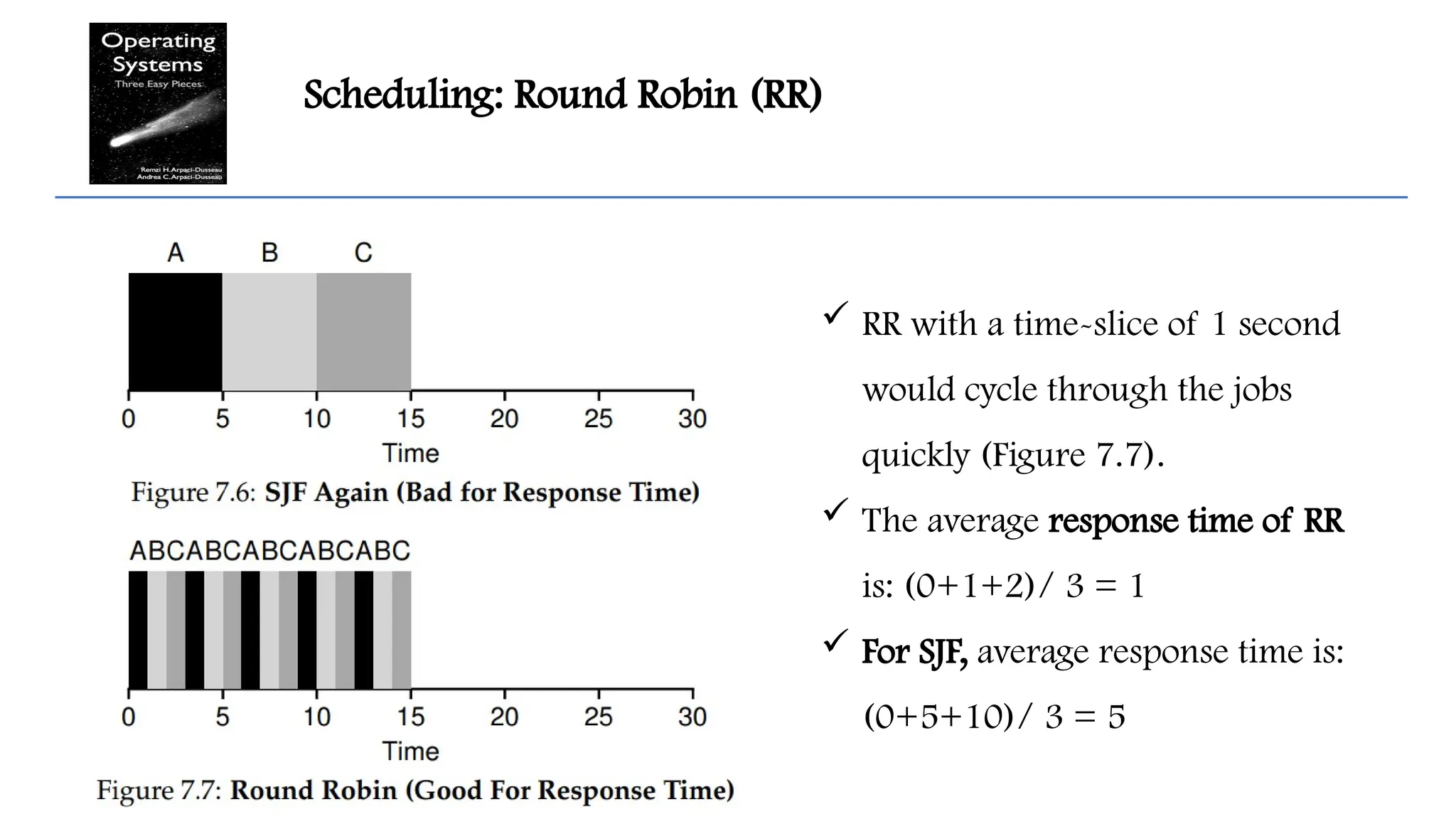
RR with a time-slice of 1 second
would cycle through the jobs
quickly (Figure 7.7).
The average response time of RR
is: (0+1+2)/ 3 = 1
For SJF, average response time is:
(0+5+10)/ 3 = 5
16.
Scheduling: Round Robin
RR is sometimes called time-slicing.
Note that the length of a time slice must be a multiple of the timer-interrupt
period
Thus if the timer interrupts every 10 milliseconds, the time slice could be 10,
20, or any other multiple of 10 ms.
17.
Scheduling: Round Robin
The shorter it is, the better the performance of RR under the response-time
metric.
However, making the time slice too short is problematic: suddenly the cost of
context switching will dominate overall performance.
Thus, deciding on the length of the time slice presents a trade-off to a system
designer, making it long enough to amortize the cost of switching without
making it so long that the system is no longer responsive.
18.
Scheduling: Incorporating I/O
First, we relax assumption 4: All jobs only use the CPU (i.e., they perform no
I/O)
A job doesn’t use the CPU during the I/O operation
Therefore, the scheduler should schedule another job on the CPU at that
time.
When I/O request is initiated, the process goes to Blocked state from the
Running state.
When the I/O is completed, an interrupt is raised. Then the OS moves that
process from Blocked State to Ready State.
19.
Scheduling: How todeal a job that performs I/O?
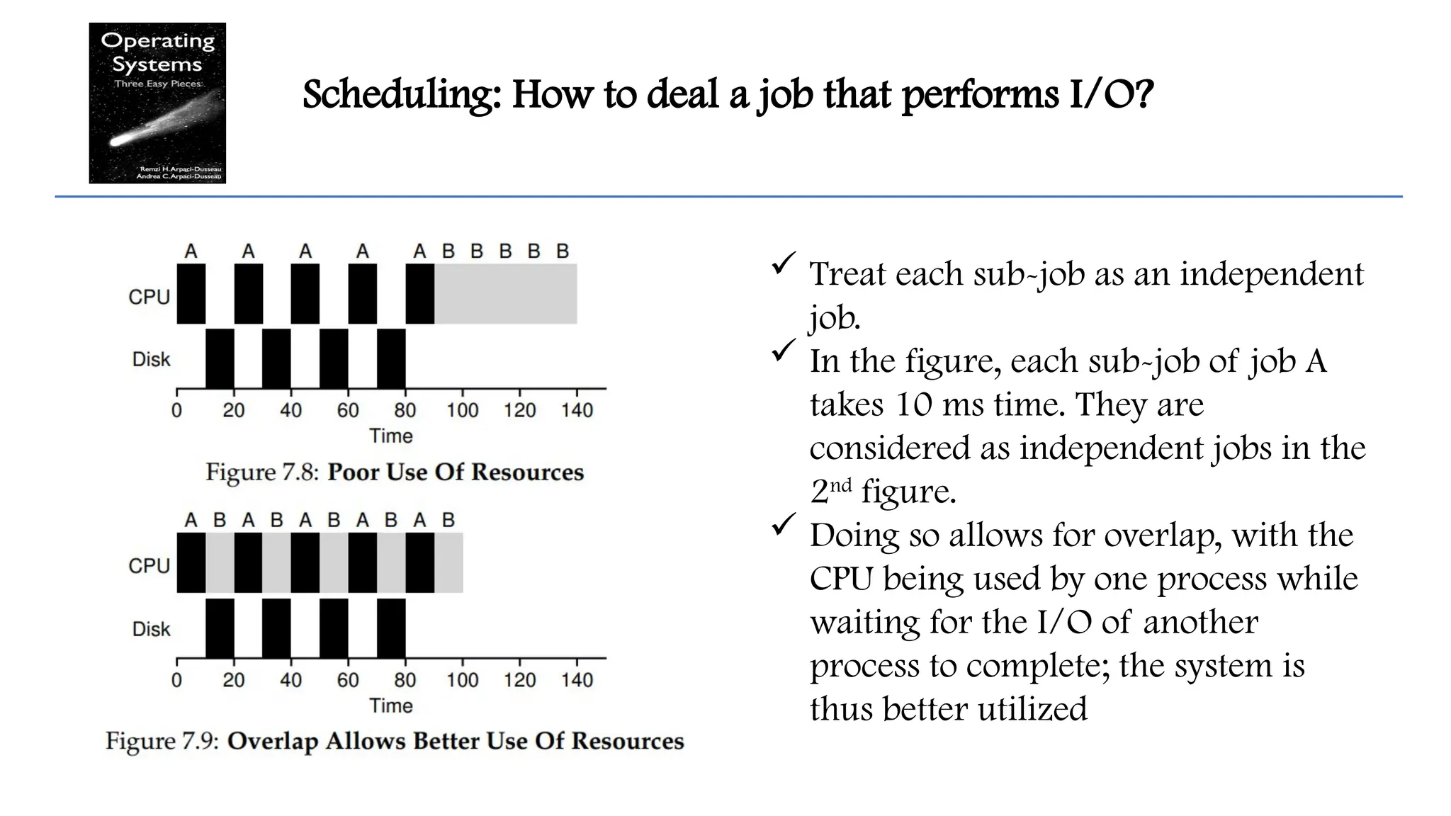
Treat each sub-job as an independent
job.
In the figure, each sub-job of job A
takes 10 ms time. They are
considered as independent jobs in the
2nd
figure.
Doing so allows for overlap, with the
CPU being used by one process while
waiting for the I/O of another
process to complete; the system is
thus better utilized
20.
Chapter 8 -Scheduling: The Multi-Level Feedback Queue
21.
THE CRUX: HOWTO SCHEDULE WITHOUT PERFECT
KNOWLEDGE?
How can we design a scheduler that both minimizes
response time for interactive jobs while also minimizing
turnaround time without a priori knowledge of job
length?
22.
THE CRUX: HOWTO SCHEDULE WITHOUT PERFECT
KNOWLEDGE?
How can we design a scheduler that both minimizes response time for interactive
jobs while also minimizing turnaround time without a priori knowledge of job
length?
The fundamental problem MLFQ tries to address is two-fold
First, it would like to optimize turnaround time, which is done by running shorter
jobs first.
Unfortunately, the OS doesn’t generally know how long a job will run for.
Second, MLFQ would like to make a system feel responsive to interactive users
(i.e., users sitting and staring at the screen, waiting for a process to finish), and
thus minimize response time
Unfortunately, algorithms like Round Robin reduce response time but are terrible
for turnaround time.
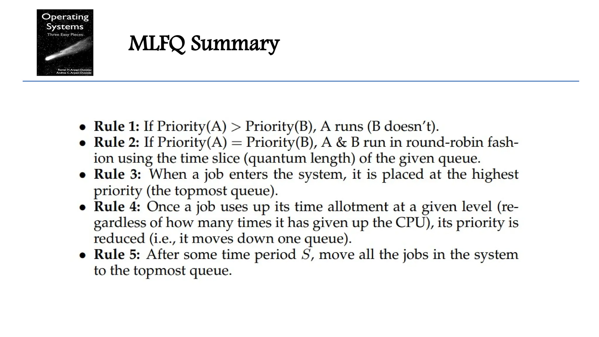
23.
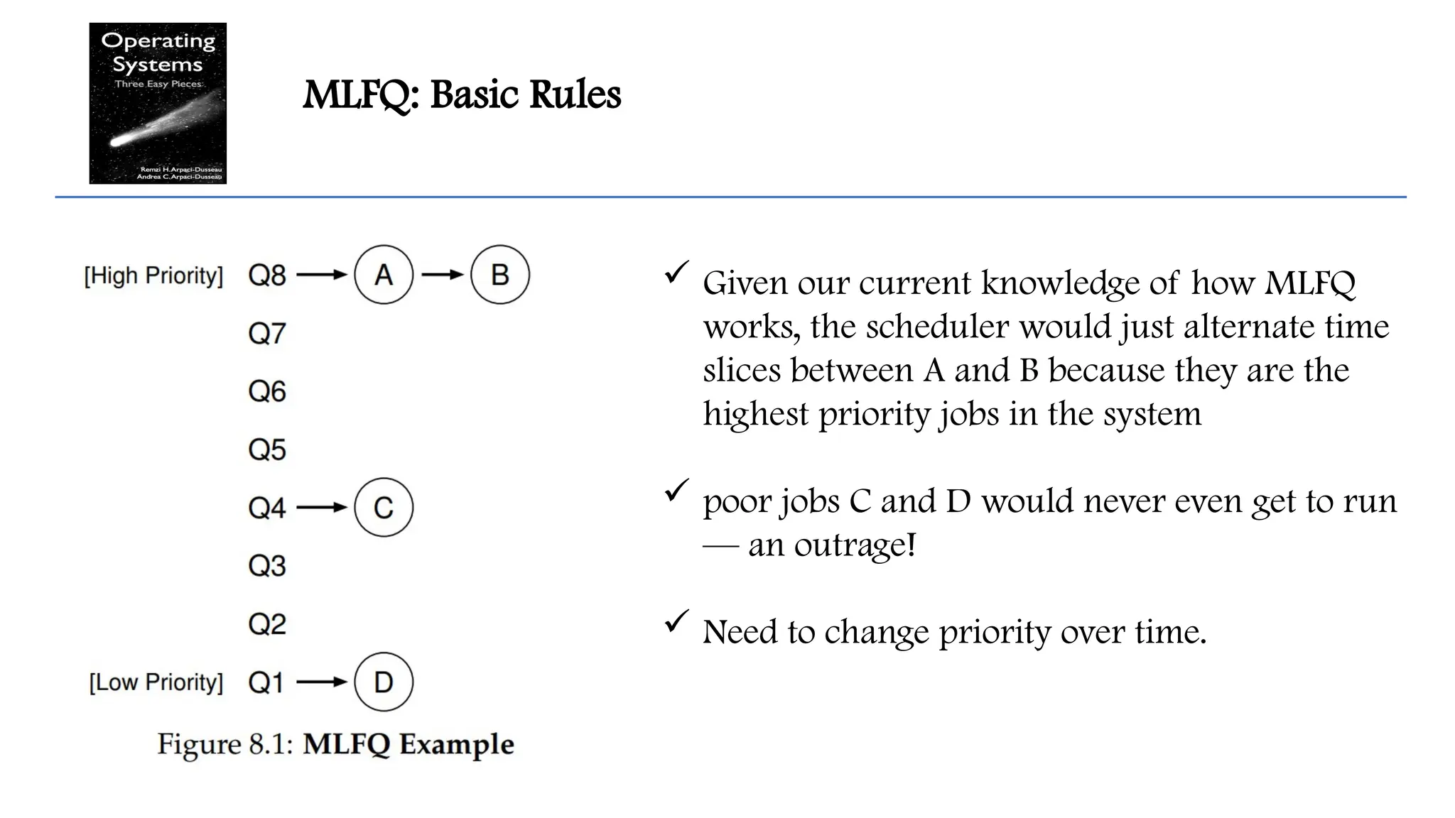
MLFQ: Basic Rules
The MLFQ has a number of distinct queues, each assigned a different priority
level.
At any given time, a job that is ready to run is on a single queue.
MLFQ uses priorities to decide which job should run at a given time: a job with
higher priority (i.e., a job on a higher queue) is chosen to run.
More than one job may be on a given queue, and thus have the same priority. In
this case, we will just use round-robin scheduling among those jobs
24.
MLFQ: Basic Rules
Rather than giving a fixed priority to each job, MLFQ varies the priority of a job
based on its observed behavior.
A job that repeatedly relinquishes CPU -> interactive job -> MLFQ will give it
higher priority
A job that uses CPU intensively for long periods of time -> MLFQ will reduce its
priority.
25.
MLFQ: Basic Rules
Given our current knowledge of how MLFQ
works, the scheduler would just alternate time
slices between A and B because they are the
highest priority jobs in the system
poor jobs C and D would never even get to run
— an outrage!
Need to change priority over time.
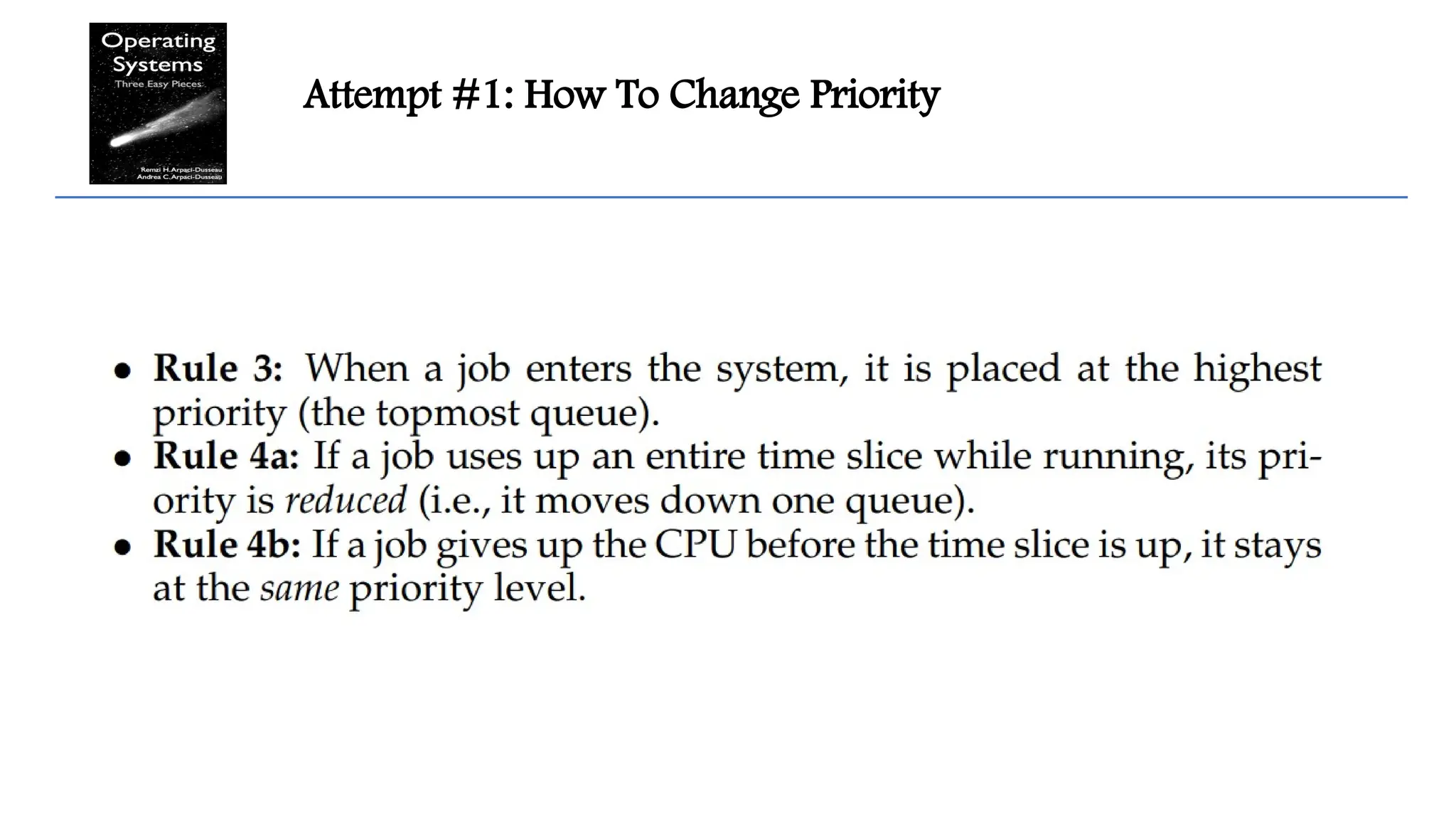
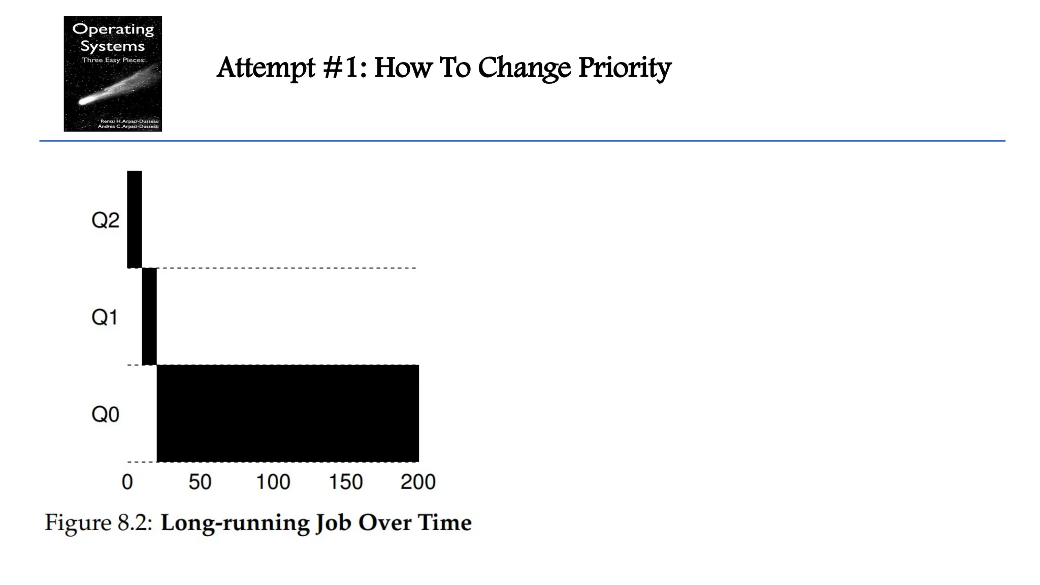
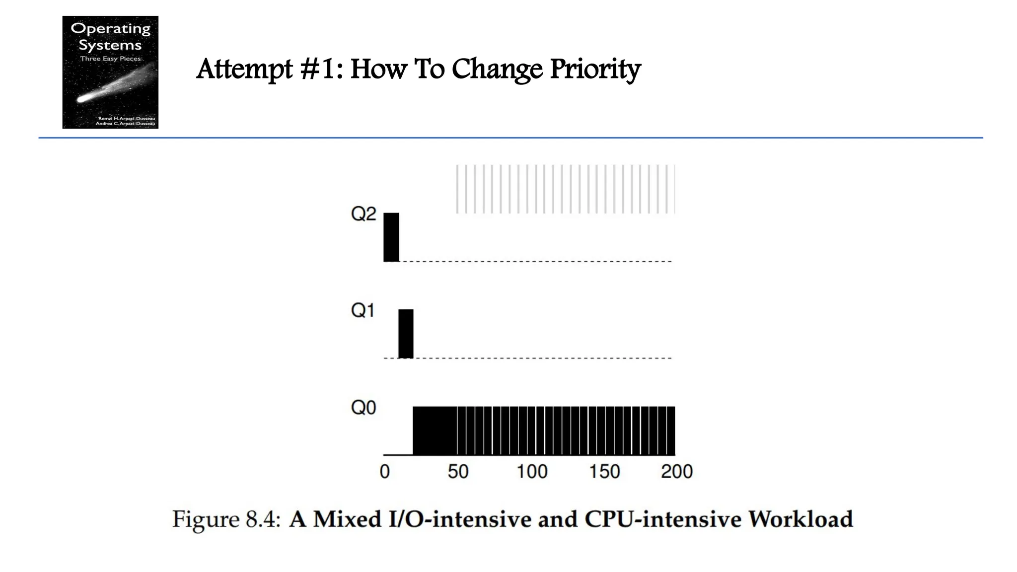
Attempt #1: HowTo Change Priority
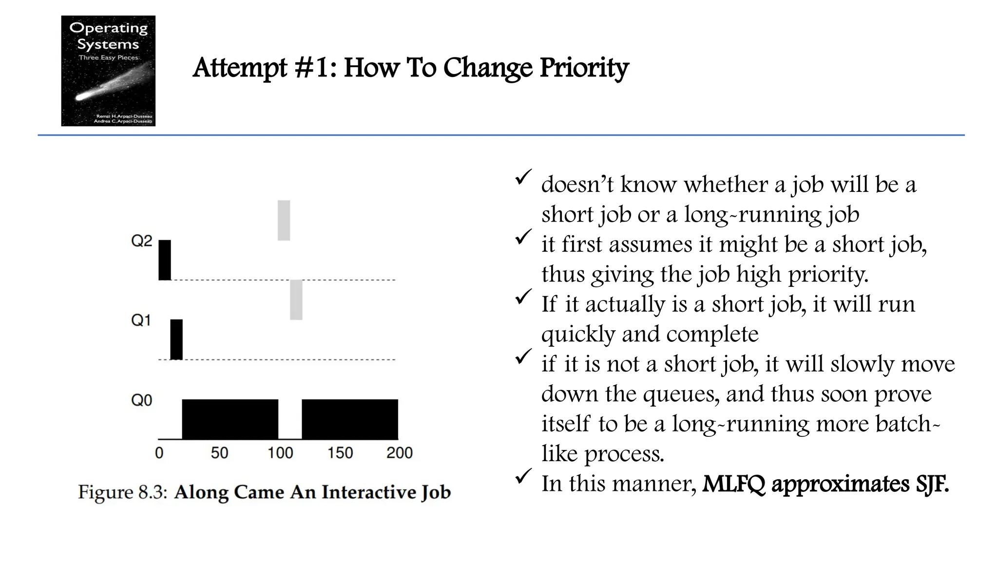
doesn’t know whether a job will be a
short job or a long-running job
it first assumes it might be a short job,
thus giving the job high priority.
If it actually is a short job, it will run
quickly and complete
if it is not a short job, it will slowly move
down the queues, and thus soon prove
itself to be a long-running more batch-
like process.
In this manner, MLFQ approximates SJF.
Problems With OurCurrent MLFQ : Starvation
if there are “too many” interactive jobs in the system, they will combine to
consume all CPU time, and thus long-running jobs will never receive any CPU
time (they starve).
We’d like to make some progress on these jobs even in this scenario.
31.
Problems With OurCurrent MLFQ : Game The Scheduler
Gaming the scheduler generally refers to the idea of doing something sneaky to
trick the scheduler into giving you more than your fair share of the resource.
Before the time slice is over, issue an I/O operation (to some file you don’t care
about) and thus relinquish the CPU
Doing so allows you to remain in the same queue, and thus gain a higher
percentage of CPU time.
When done right (e.g., by running for 99% of a time slice before relinquishing
the CPU), a job could nearly monopolize the CPU.
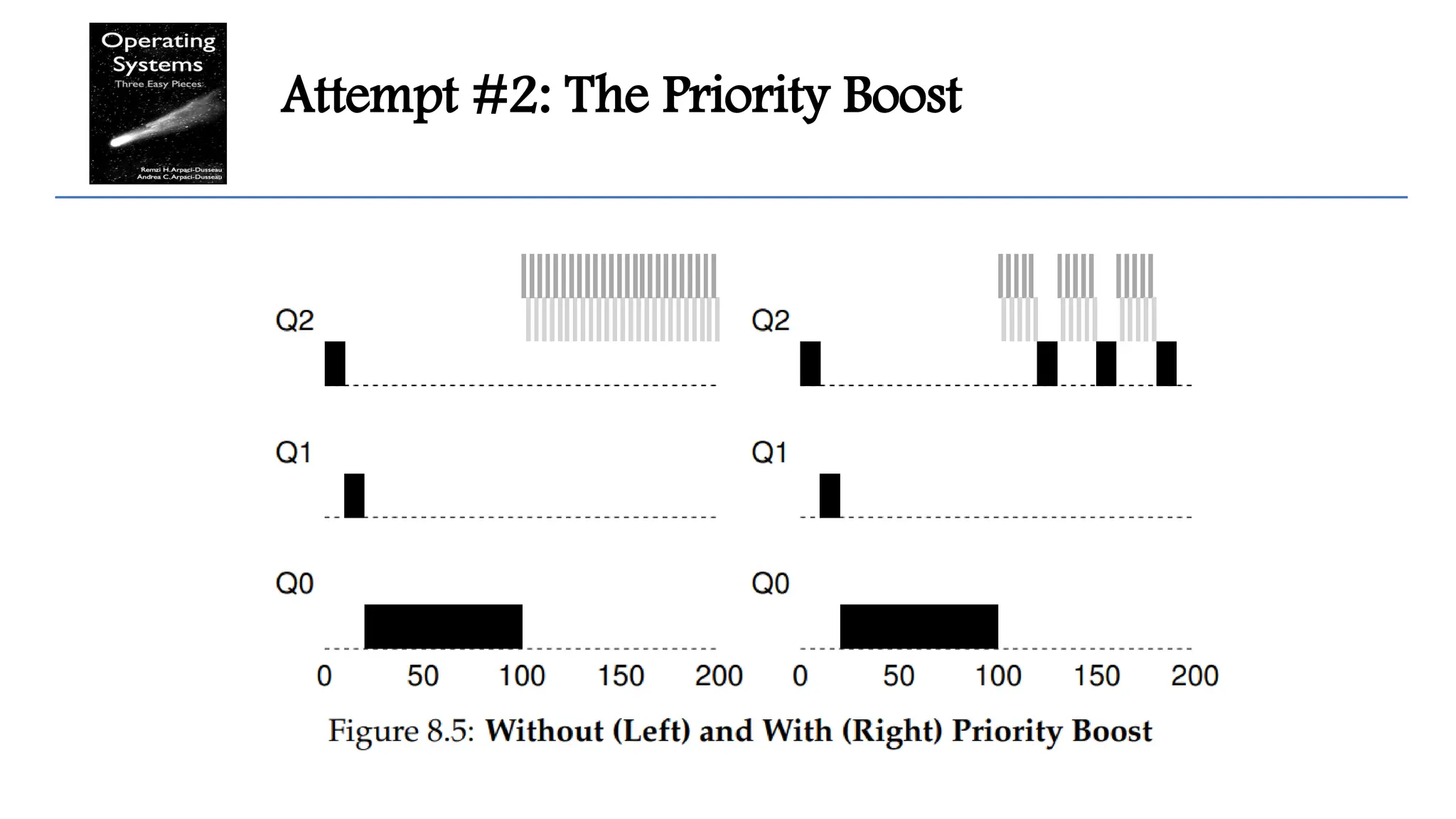
32.
Attempt #2: ThePriority Boost
To avoid the problem of starvation, periodically boost the priority of all the jobs
in system.
Our new rule solves two problems at once.
First, processes are guaranteed not to starve: by sitting in the top queue, a job will
share the CPU with other high-priority jobs in a round-robin fashion, and thus
eventually receive service.
Second, if a CPU-bound job has become interactive, the scheduler treats it properly
once it has received the priority boost.
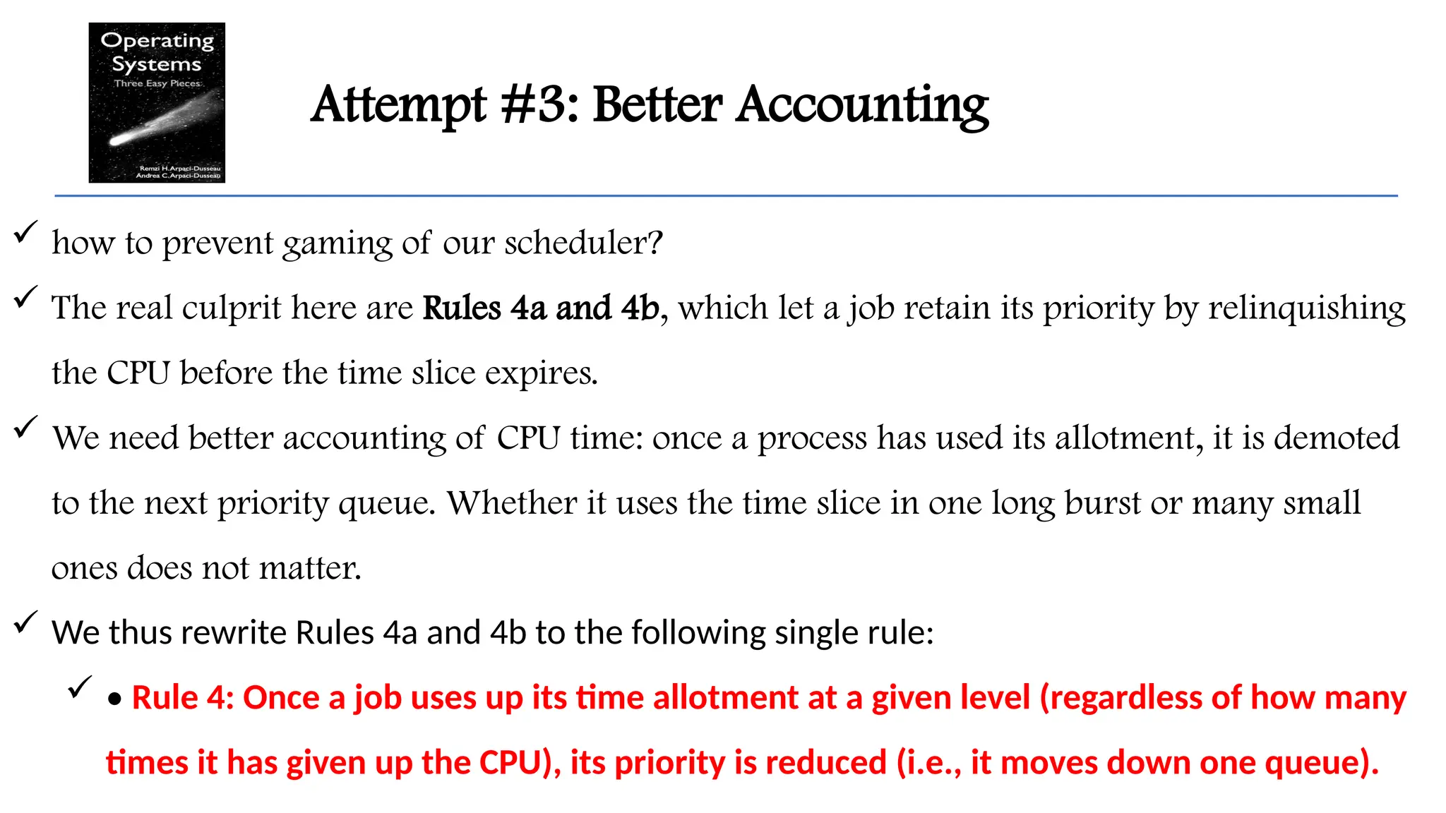
Attempt #3: BetterAccounting
how to prevent gaming of our scheduler?
The real culprit here are Rules 4a and 4b, which let a job retain its priority by relinquishing
the CPU before the time slice expires.
We need better accounting of CPU time: once a process has used its allotment, it is demoted
to the next priority queue. Whether it uses the time slice in one long burst or many small
ones does not matter.
We thus rewrite Rules 4a and 4b to the following single rule:
• Rule 4: Once a job uses up its time allotment at a given level (regardless of how many
times it has given up the CPU), its priority is reduced (i.e., it moves down one queue).