This document summarizes that some slides were adapted from various sources including machine learning lectures and professors from Stanford University, Cornell University, IIT Kharagpur, and University of Illinois at Chicago. Students are requested to use this material for study purposes only and not distribute it.
![• Let’s consider D, the entire distribution of data, and T, the training
set.
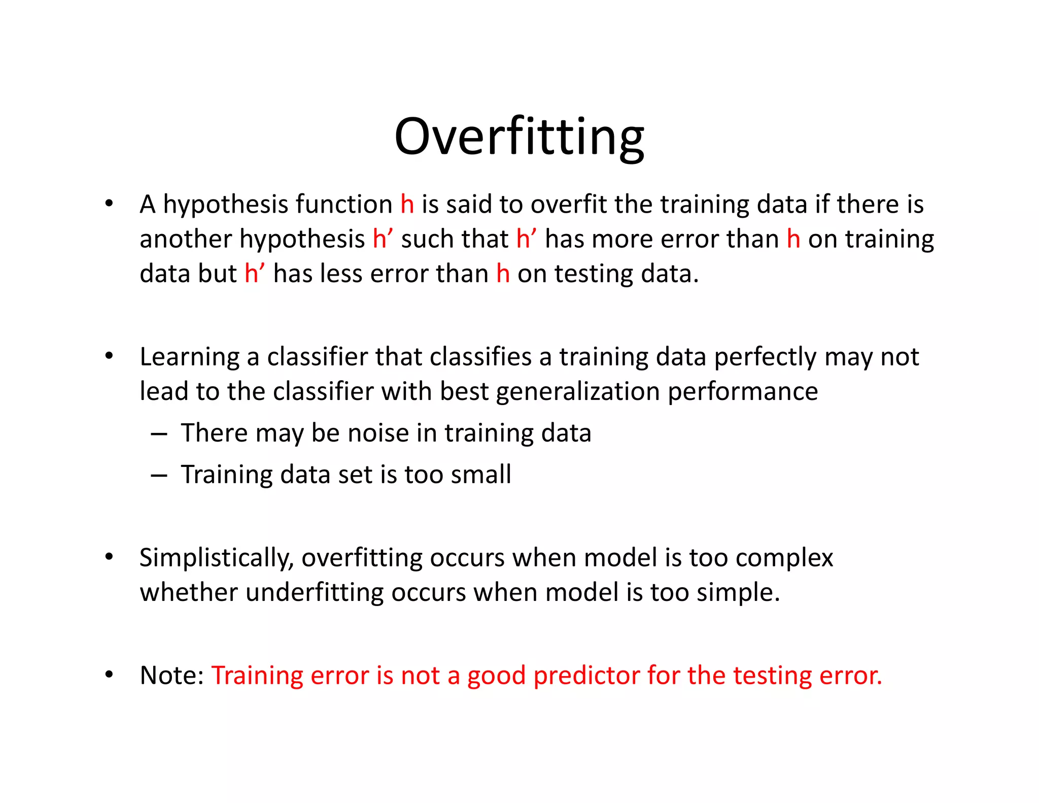
• Hypothesis h H overfits D if
h’ h H such that
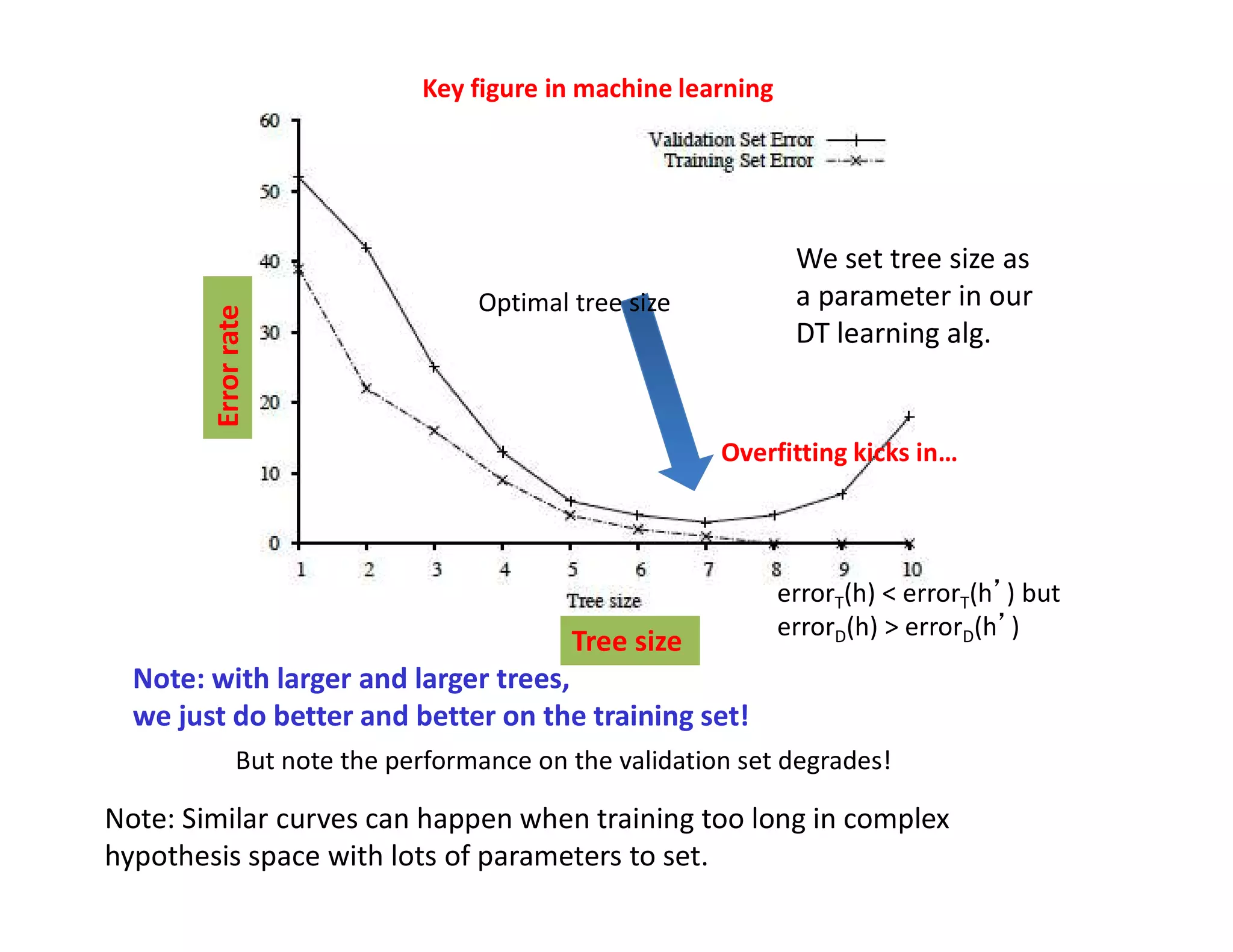
(1) errorT(h) < errorT(h’) [i.e. doing well on training set]
but
(2) errorD(h) > errorD(h’)
•What do we care about most (1) or (2)?
•Estimate error on full distribution by using test data set.
Error on test data: Generalization error (want it low!!)
•Generalization to unseen examples/data is what we care about.
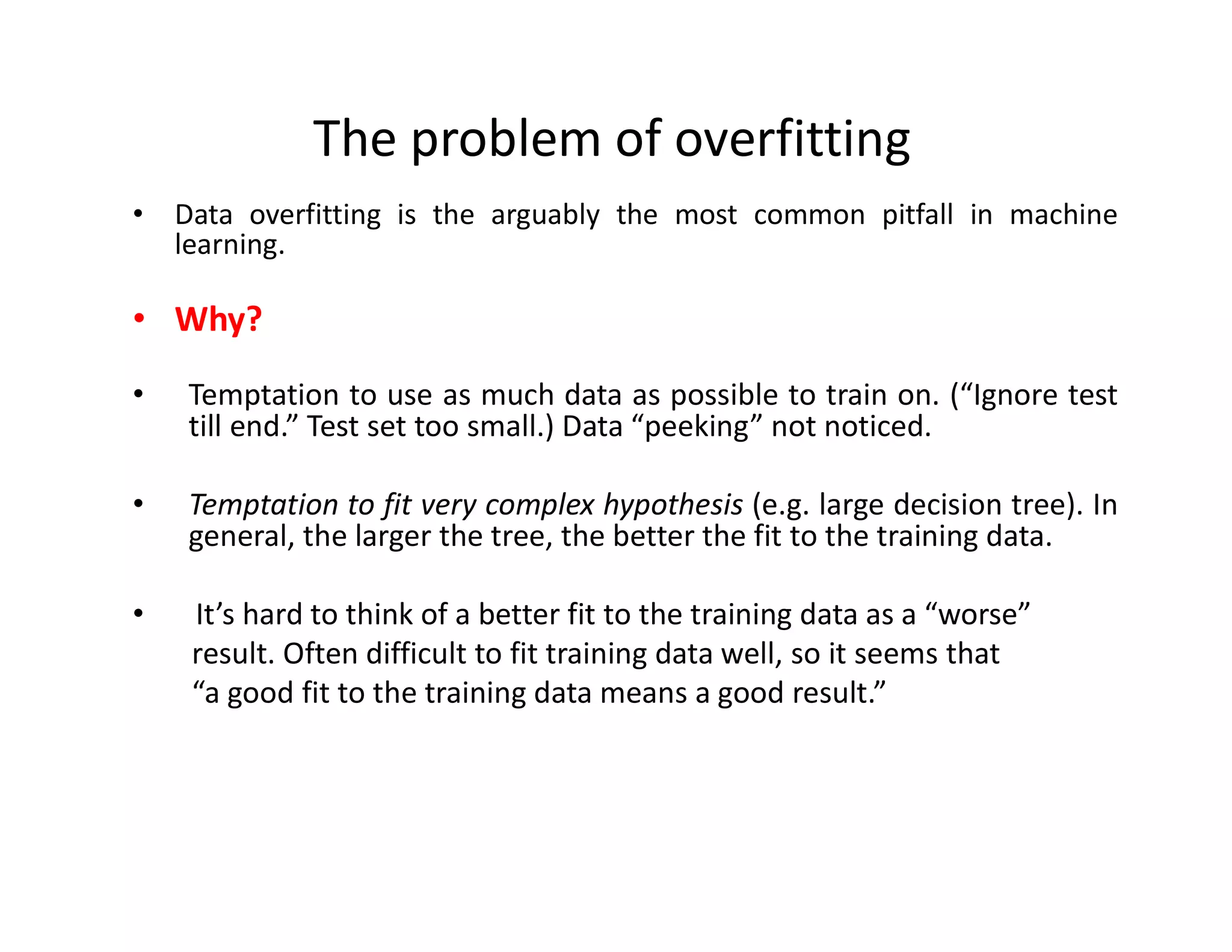
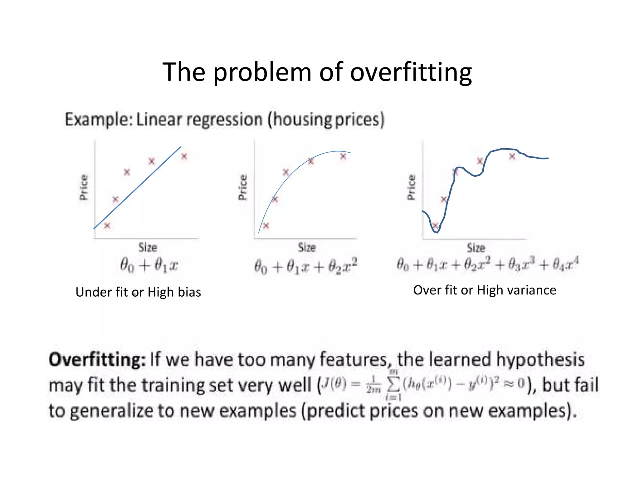
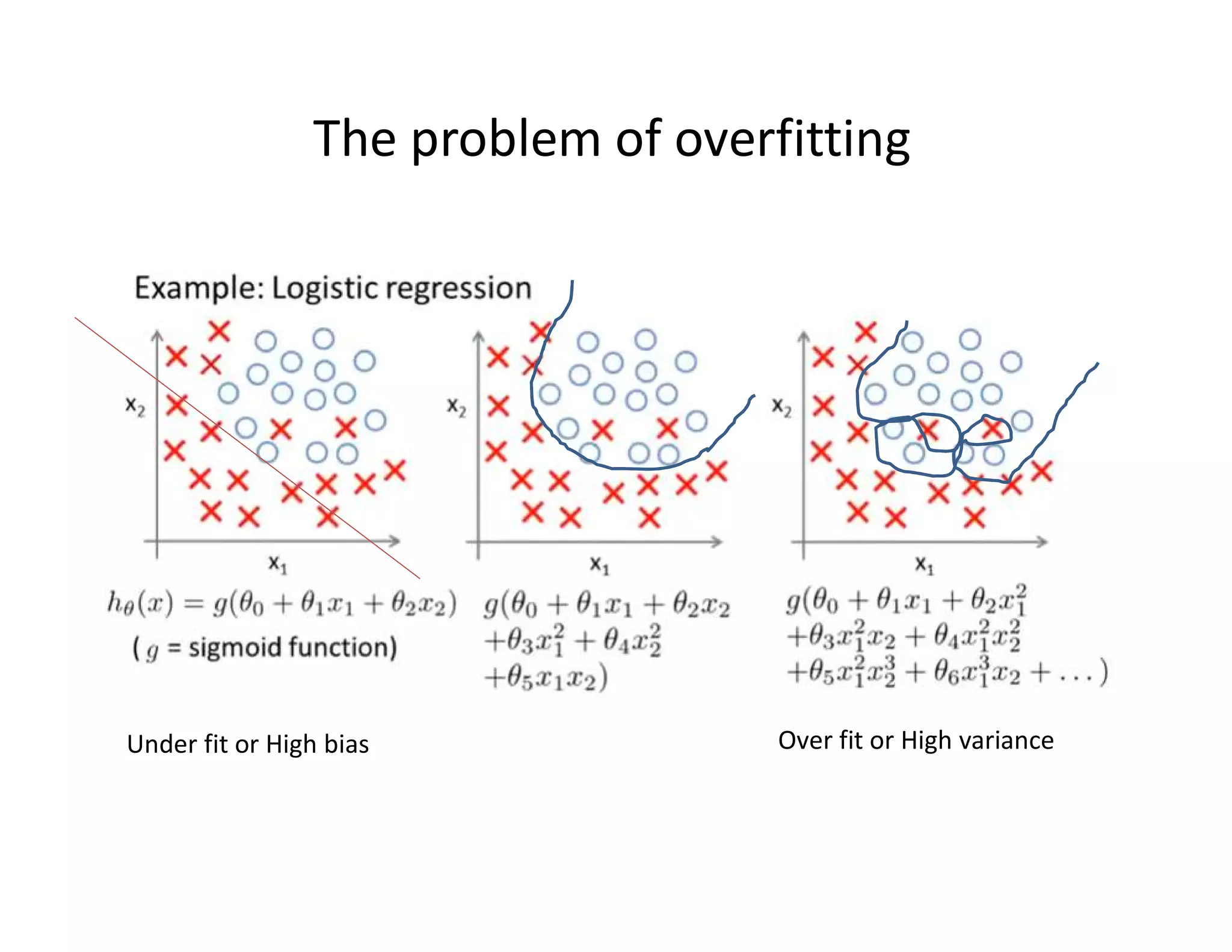
The problem of overfitting](https://image.slidesharecdn.com/l1intro2supervisedlearning-211117120740/75/L1-intro2-supervised_learning-51-2048.jpg)