Introduction to Huffman_Coding algorithm.ppt

Huffman Coding
Vida Movahedi
October 2006

Contents
• A simple example
• Definitions
• Huffman Coding Algorithm
• Image Compression

A simple example
• Suppose we have a message consisting of 5 symbols,
e.g. [►♣♣♠☻►♣☼►☻]
• How can we code this message using 0/1 so the coded
message will have minimum length (for transmission or
saving!)
• 5 symbols  at least 3 bits
• For a simple encoding,
length of code is 10*3=30 bits

A simple example – cont.
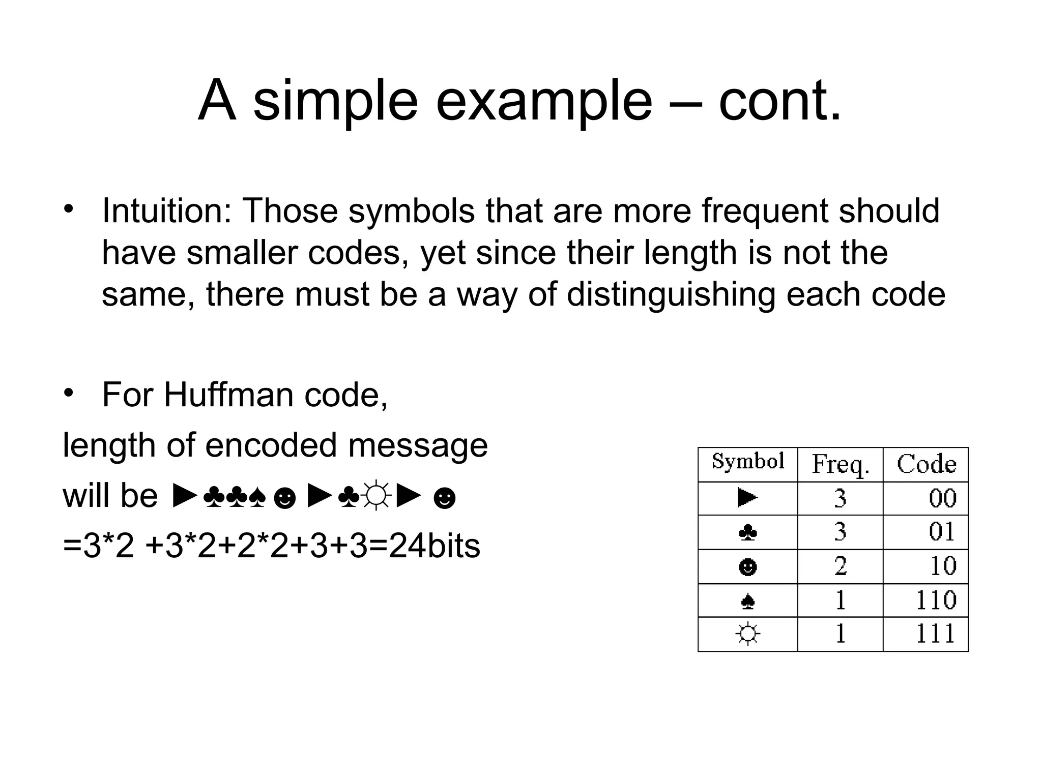
• Intuition: Those symbols that are more frequent should
have smaller codes, yet since their length is not the
same, there must be a way of distinguishing each code
• For Huffman code,
length of encoded message
will be ►♣♣♠☻►♣☼►☻
=3*2 +3*2+2*2+3+3=24bits

Definitions
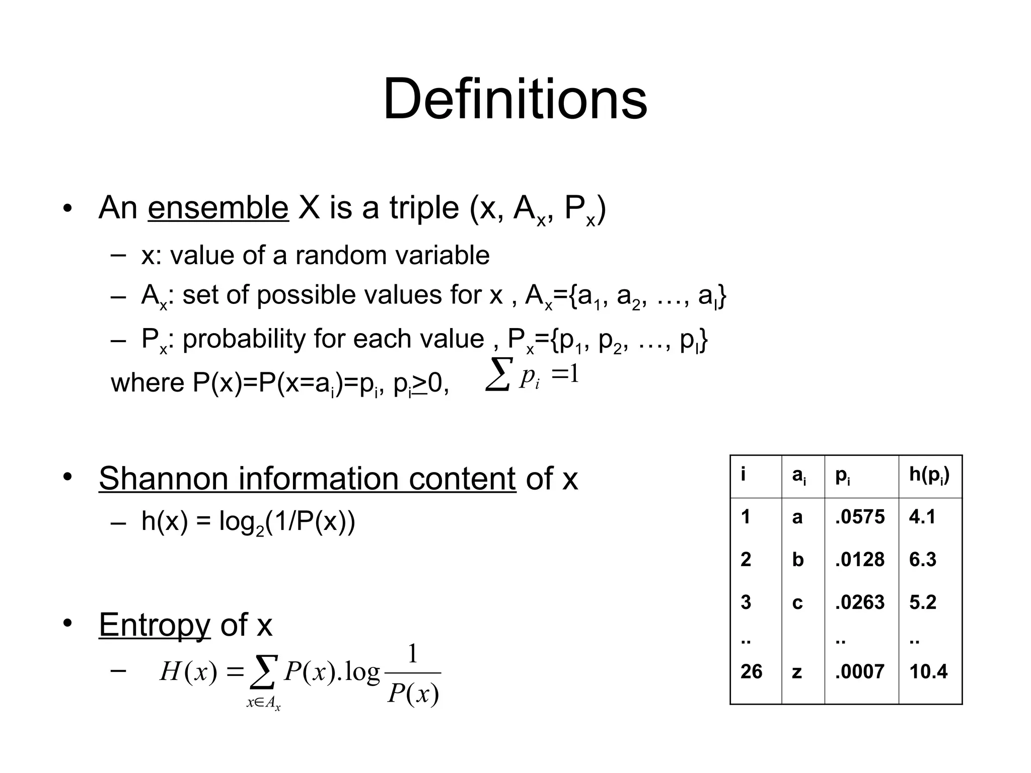
• An ensemble X is a triple (x, Ax, Px)
– x: value of a random variable
– Ax: set of possible values for x , Ax={a1, a2, …, aI}
– Px: probability for each value , Px={p1, p2, …, pI}
where P(x)=P(x=ai)=pi, pi>0,
• Shannon information content of x
– h(x) = log2(1/P(x))
• Entropy of x
–
1

 i
p



x
A
x x
P
x
P
x
H
)
(
1
log
).
(
)
(
i ai pi h(pi)
1 a .0575 4.1
2 b .0128 6.3
3 c .0263 5.2
.. .. ..
26 z .0007 10.4

Source Coding Theorem
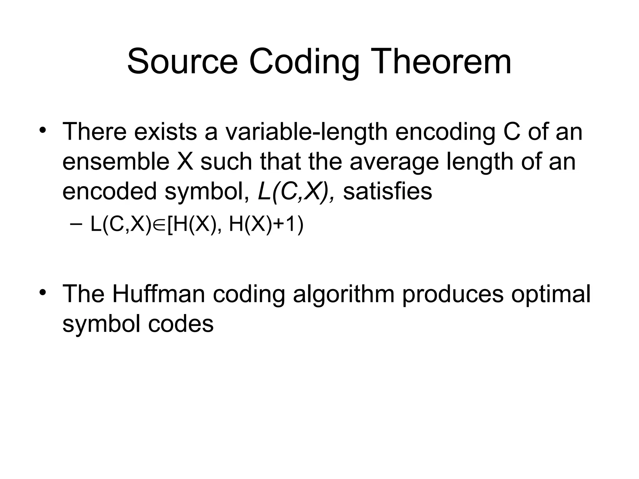
• There exists a variable-length encoding C of an
ensemble X such that the average length of an
encoded symbol, L(C,X), satisfies
– L(C,X)[H(X), H(X)+1)
• The Huffman coding algorithm produces optimal
symbol codes

Symbol Codes
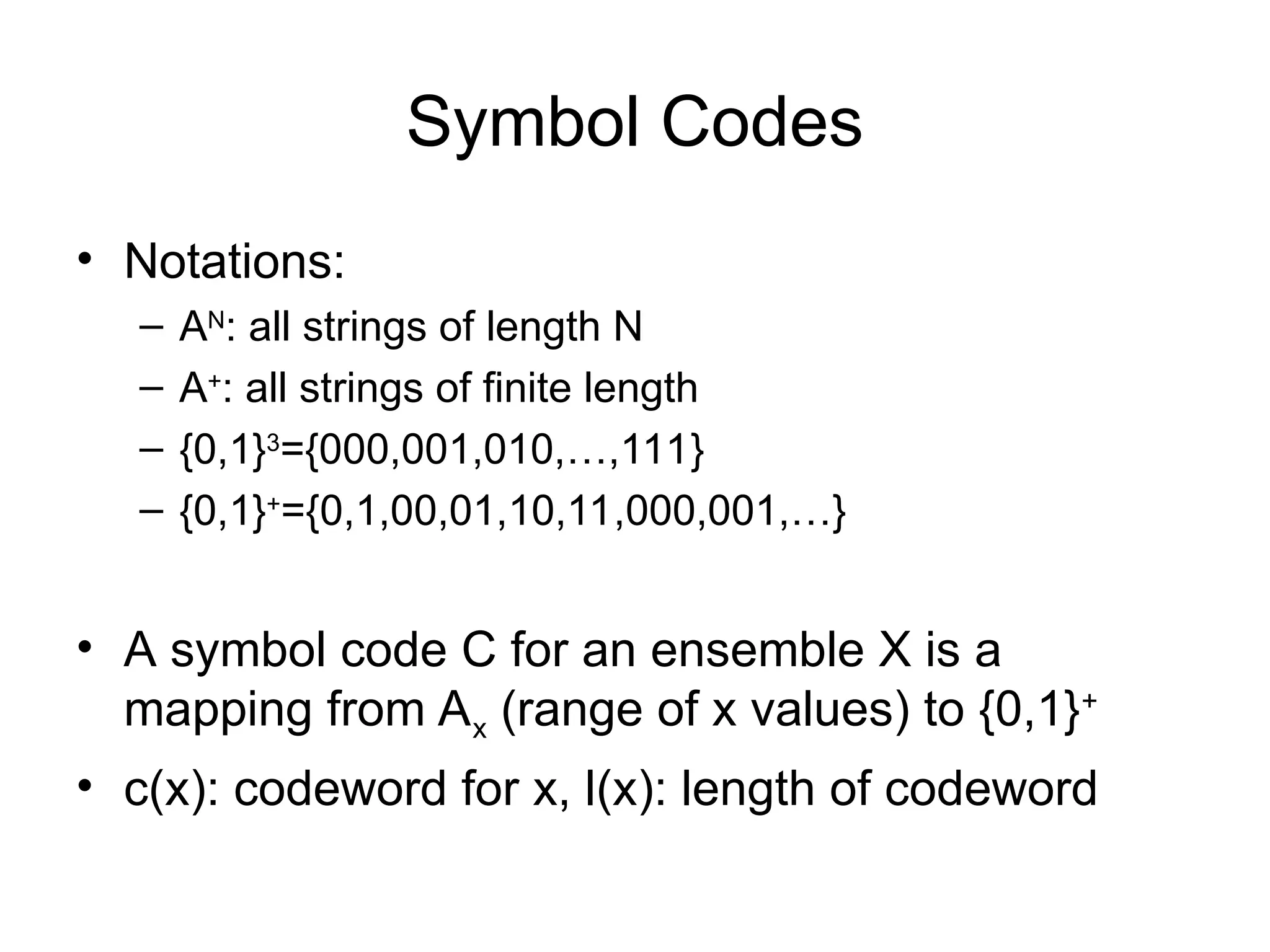
• Notations:
– AN
: all strings of length N
– A+
: all strings of finite length
– {0,1}3
={000,001,010,…,111}
– {0,1}+
={0,1,00,01,10,11,000,001,…}
• A symbol code C for an ensemble X is a
mapping from Ax (range of x values) to {0,1}+
• c(x): codeword for x, l(x): length of codeword

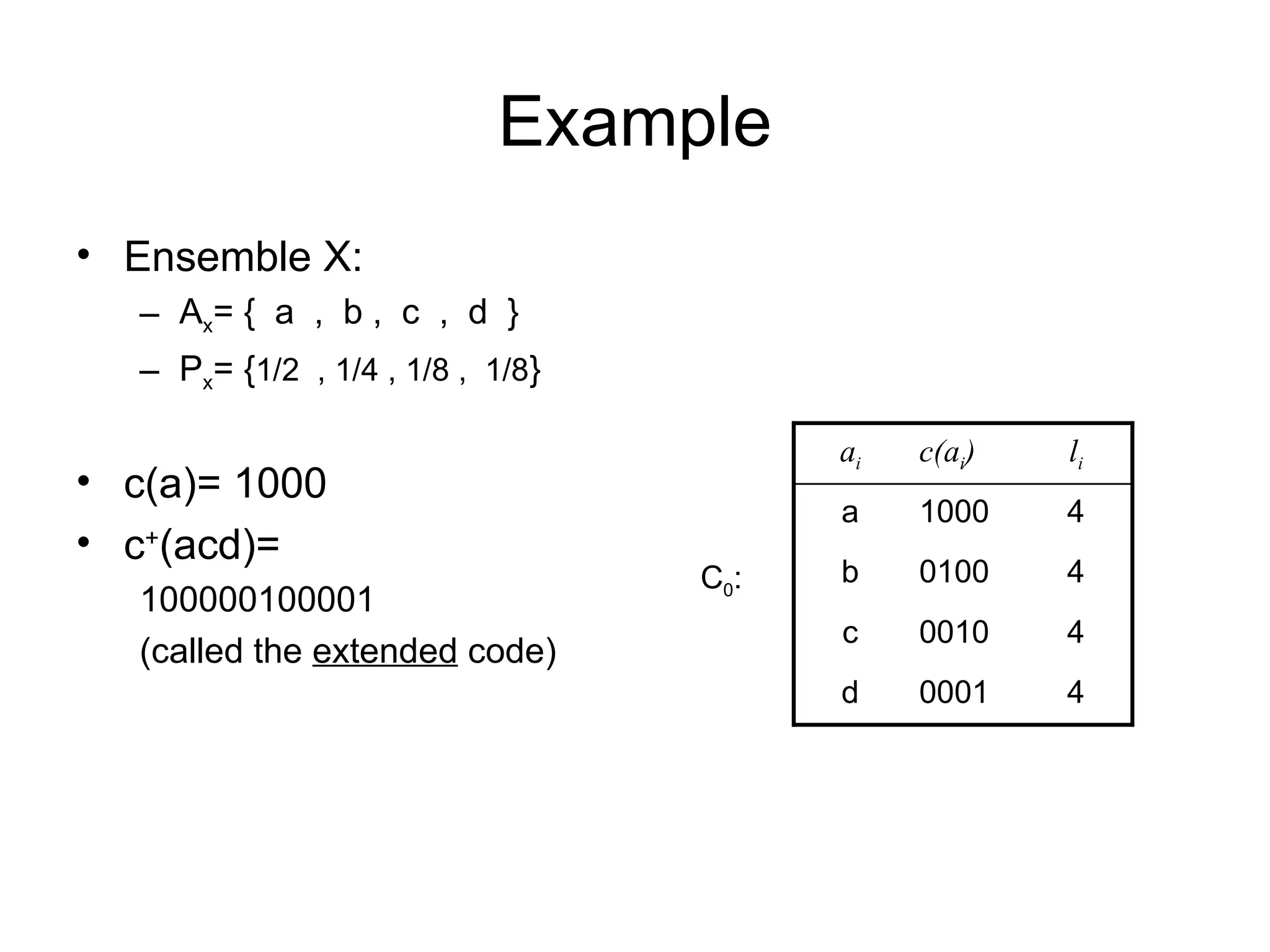
Example
• Ensemble X:
– Ax= { a , b , c , d }
– Px= {1/2 , 1/4 , 1/8 , 1/8}
• c(a)= 1000
• c+
(acd)=
100000100001
(called the extended code)
4
0001
d
4
0010
c
4
0100
b
4
1000
a
li
c(ai)
ai
C0:

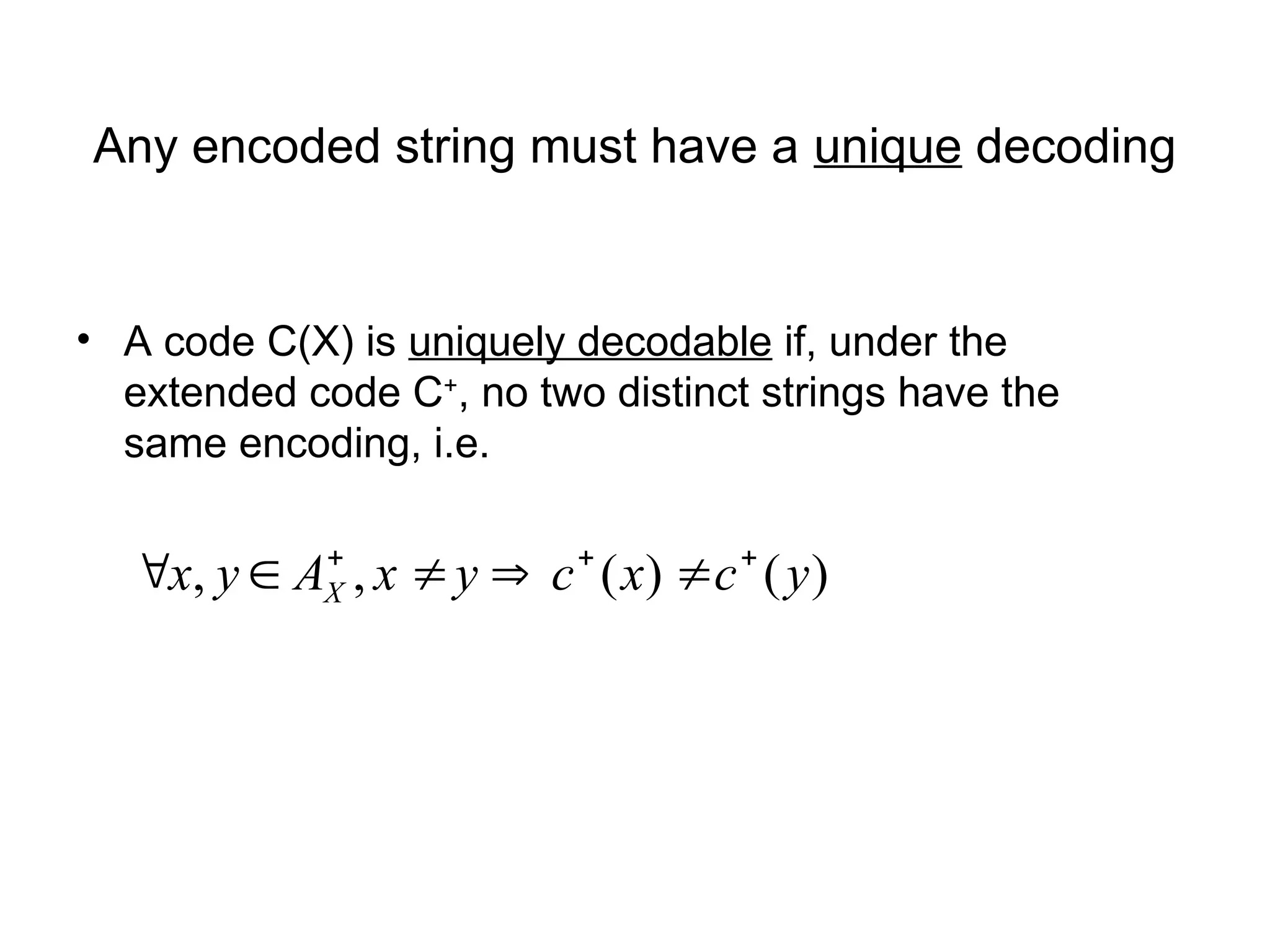
Any encoded string must have a unique decoding
• A code C(X) is uniquely decodable if, under the
extended code C+
, no two distinct strings have the
same encoding, i.e.
)
(
)
(
,
, y
c
x
c
y
x
A
y
x X









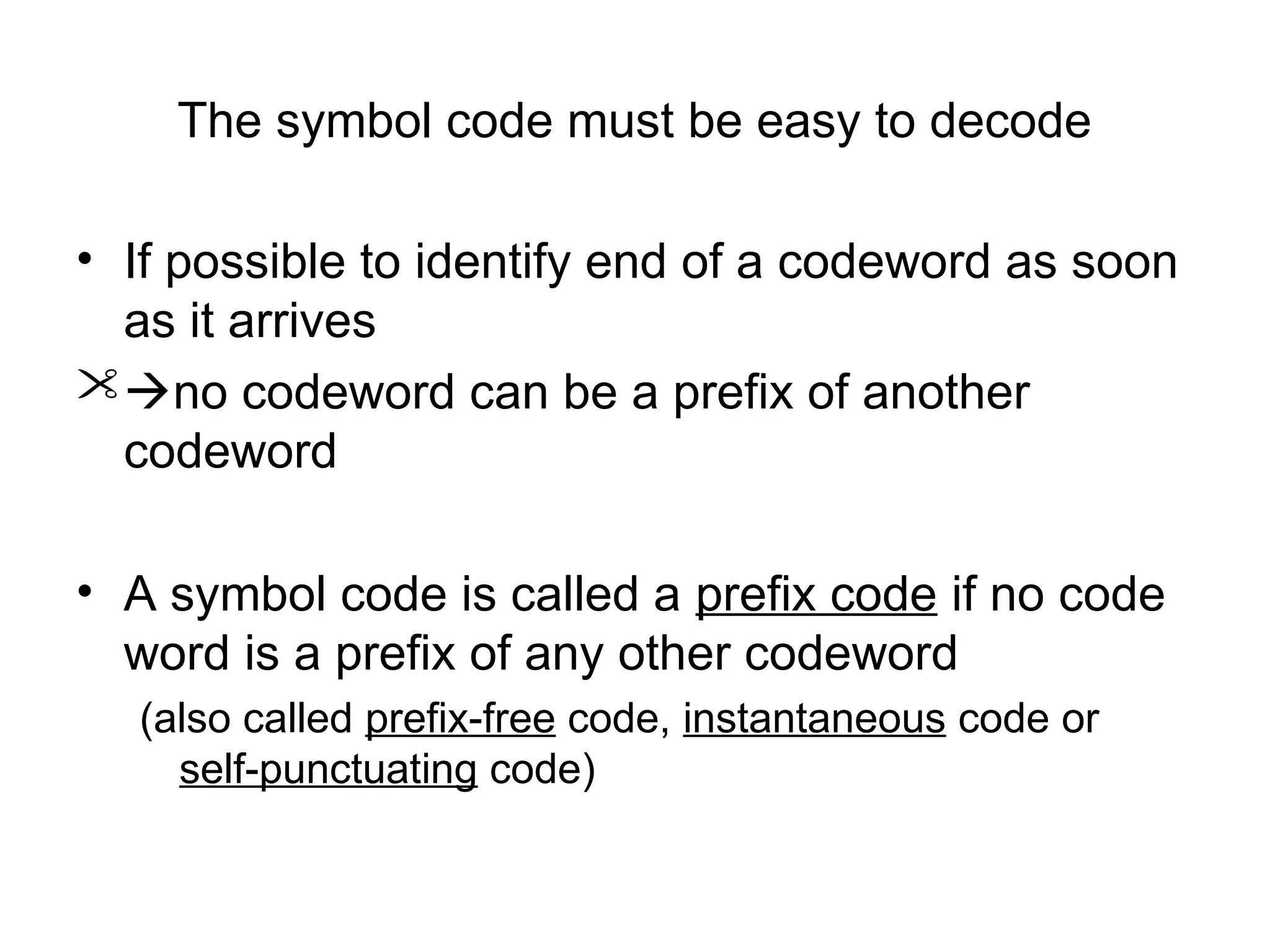
The symbol code must be easy to decode
• If possible to identify end of a codeword as soon
as it arrives
no codeword can be a prefix of another
codeword
• A symbol code is called a prefix code if no code
word is a prefix of any other codeword
(also called prefix-free code, instantaneous code or
self-punctuating code)

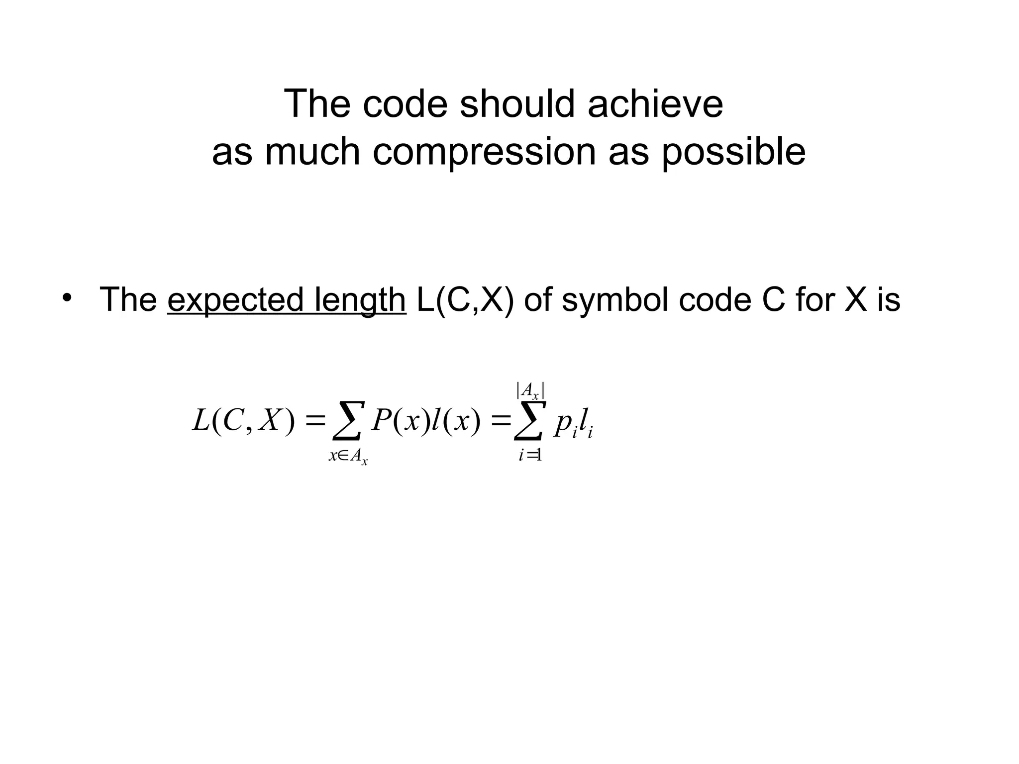
The code should achieve
as much compression as possible
• The expected length L(C,X) of symbol code C for X is

 



|
|
1
)
(
)
(
)
,
(
x
x
A
i
i
i
A
x
l
p
x
l
x
P
X
C
L

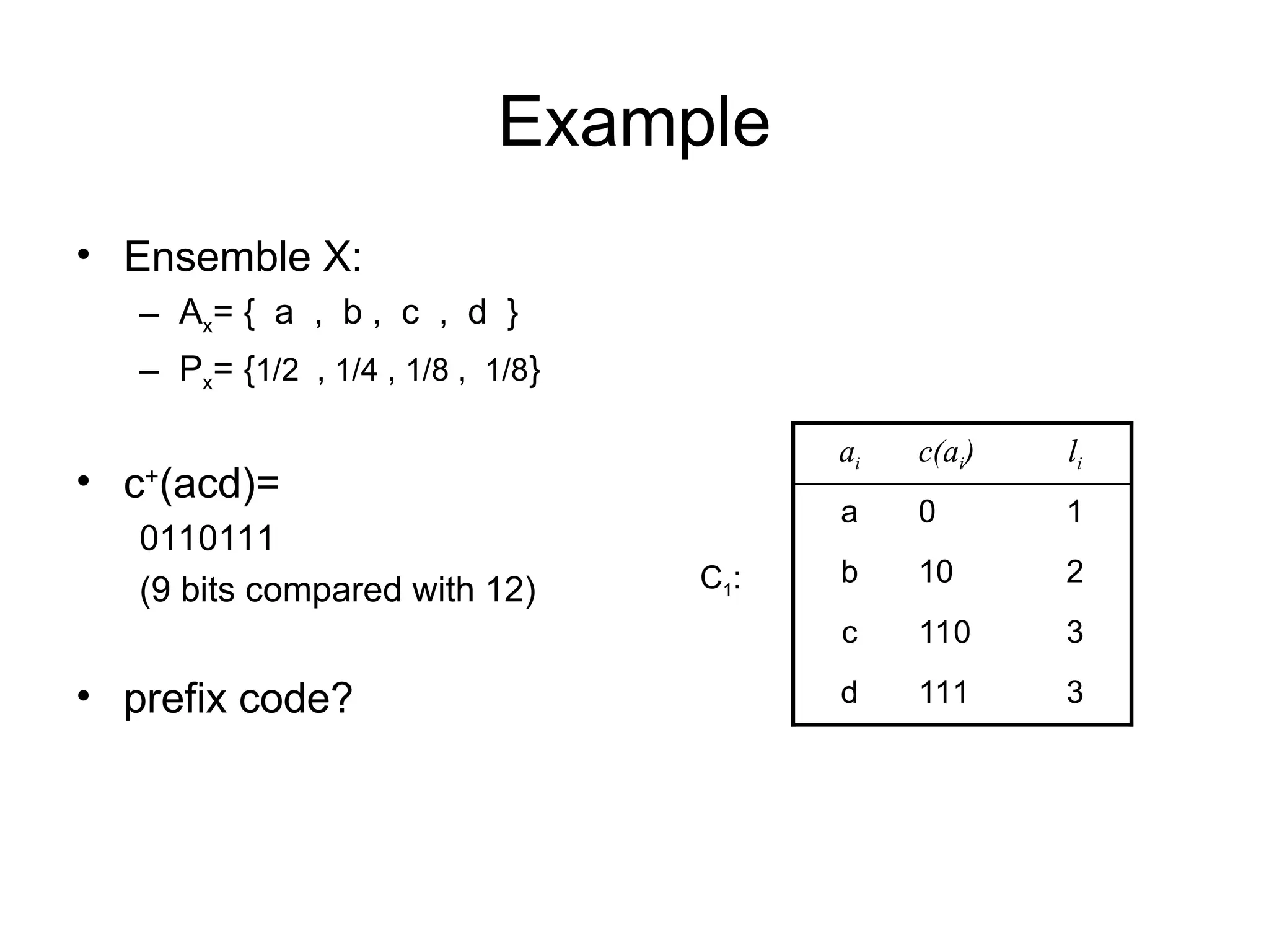
Example
• Ensemble X:
– Ax= { a , b , c , d }
– Px= {1/2 , 1/4 , 1/8 , 1/8}
• c+
(acd)=
0110111
(9 bits compared with 12)
• prefix code? 3
111
d
3
110
c
2
10
b
1
0
a
li
c(ai)
ai
C1:

The Huffman Coding algorithm- History
• In 1951, David Huffman and his MIT information theory
classmates given the choice of a term paper or a final
exam
• Huffman hit upon the idea of using a frequency-sorted
binary tree and quickly proved this method the most
efficient.
• In doing so, the student outdid his professor, who had
worked with information theory inventor Claude Shannon
to develop a similar code.
• Huffman built the tree from the bottom up instead of from
the top down

Huffman Coding Algorithm
1. Take the two least probable symbols in the
alphabet
(longest codewords, equal length, differing in last digit)
2. Combine these two symbols into a single
symbol, and repeat.

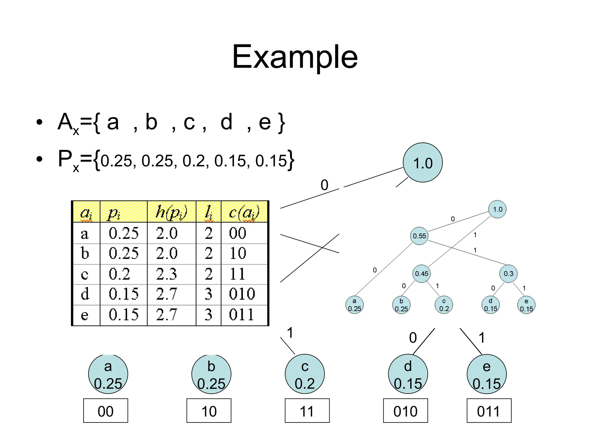
Example
• Ax={ a , b , c , d , e }
• Px={0.25, 0.25, 0.2, 0.15, 0.15}
d
0.15
e
0.15
b
0.25
c
0.2
a
0.25
0.3
0 1
0.45
0 1
0.55
0
1
1.0
0
1
00 10 11 010 011

Statements
• Lower bound on expected length is H(X)
• There is no better symbol code for a source
than the Huffman code
• Constructing a binary tree top-down is
suboptimal

Disadvantages of the Huffman Code
• Changing ensemble
– If the ensemble changes the frequencies and probabilities
change  the optimal coding changes
– e.g. in text compression symbol frequencies vary with context
– Re-computing the Huffman code by running through the entire
file in advance?!
– Saving/ transmitting the code too?!
• Does not consider ‘blocks of symbols’
– ‘strings_of_ch’ the next nine symbols are predictable
‘aracters_’ , but bits are used without conveying any new
information

Variations
• n-ary Huffman coding
– Uses {0, 1, .., n-1} (not just {0,1})
• Adaptive Huffman coding
– Calculates frequencies dynamically based on recent
actual frequencies
• Huffman template algorithm
– Generalizing
• probabilities  any weight
• Combining methods (addition)  any function
– Can solve other min. problems e.g. max [wi+length(ci)]

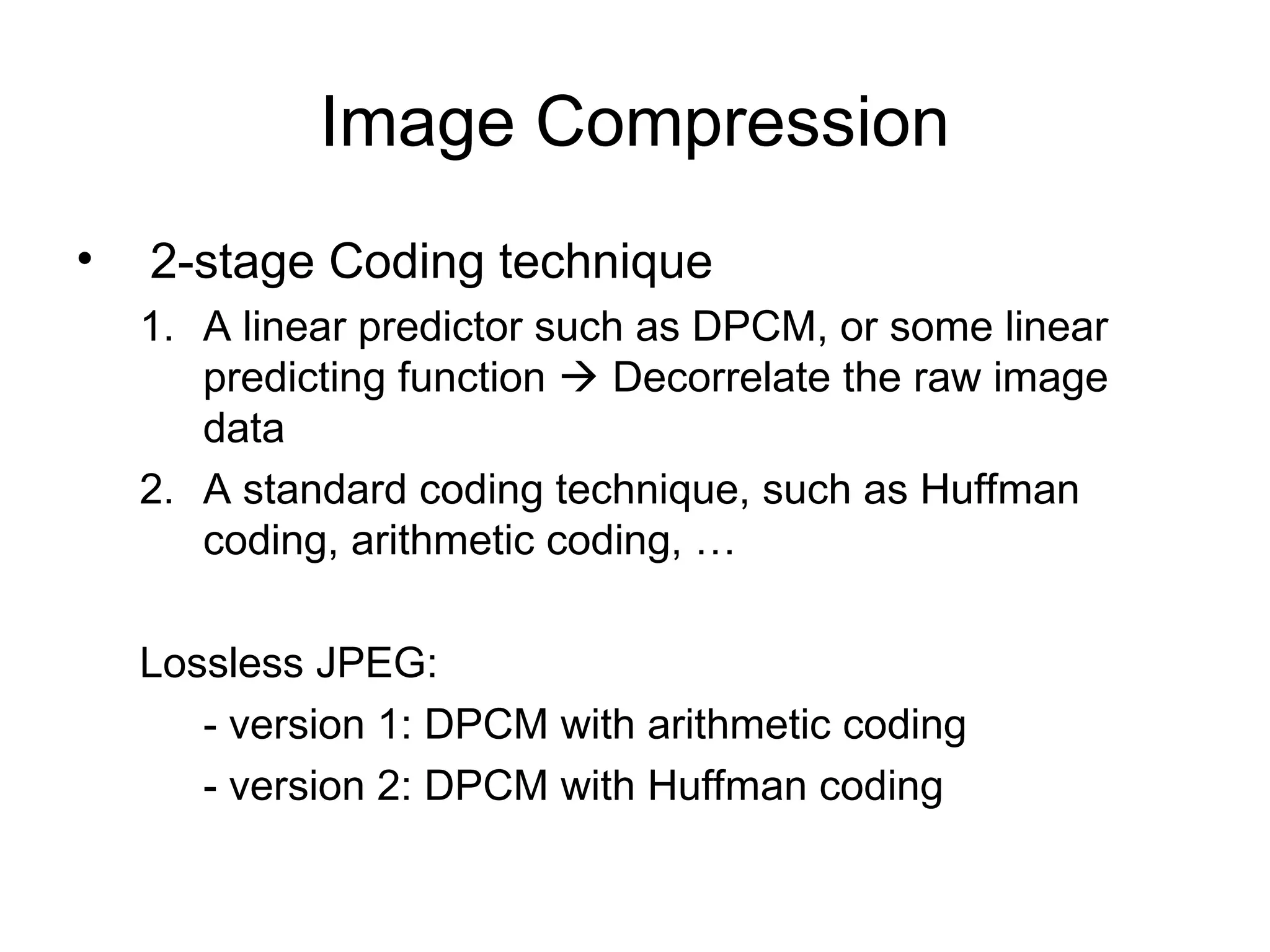
Image Compression
• 2-stage Coding technique
1. A linear predictor such as DPCM, or some linear
predicting function  Decorrelate the raw image
data
2. A standard coding technique, such as Huffman
coding, arithmetic coding, …
Lossless JPEG:
- version 1: DPCM with arithmetic coding
- version 2: DPCM with Huffman coding

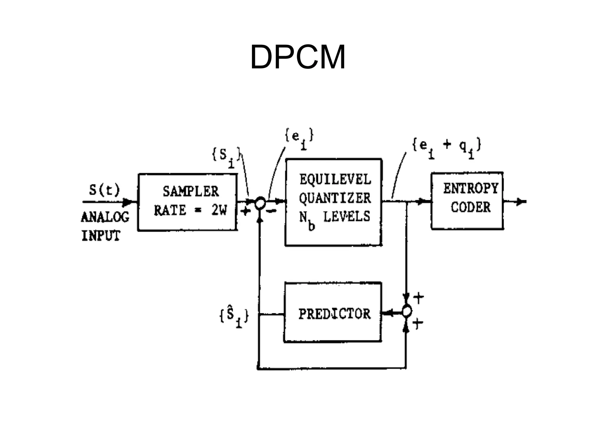
DPCM
Differential Pulse Code Modulation
• DPCM is an efficient way to encode highly
correlated analog signals into binary form
suitable for digital transmission, storage, or input
to a digital computer
• Patent by Cutler (1952)

Huffman Coding Algorithm
for Image Compression
• Step 1. Build a Huffman tree by sorting the
histogram and successively combine the two
bins of the lowest value until only one bin
remains.
• Step 2. Encode the Huffman tree and save the
Huffman tree with the coded value.
• Step 3. Encode the residual image.

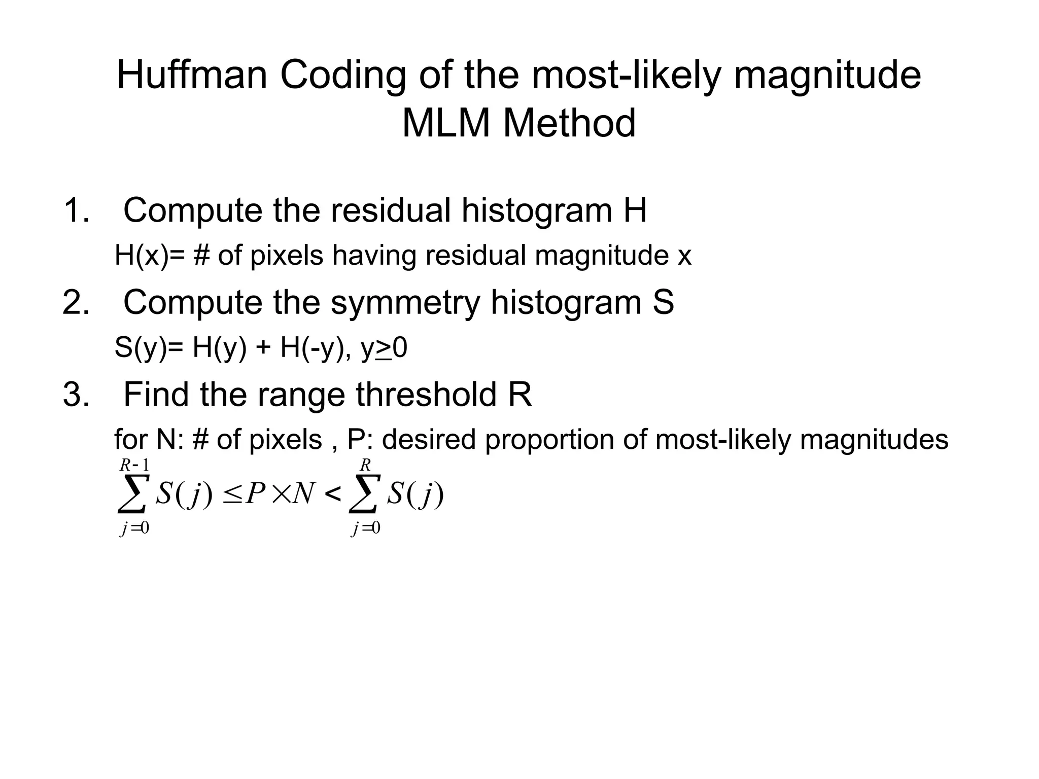
Huffman Coding of the most-likely magnitude
MLM Method
1. Compute the residual histogram H
H(x)= # of pixels having residual magnitude x
2. Compute the symmetry histogram S
S(y)= H(y) + H(-y), y>0
3. Find the range threshold R
for N: # of pixels , P: desired proportion of most-likely magnitudes

 





R
j
R
j
j
S
N
P
j
S
0
1
0
)
(
)
(

References
(1) MacKay, D.J.C. , Information Theory,
Inference, and Learning Algorithms, Cambridge
University Press, 2003.
(2) Wikipedia,
http://en.wikipedia.org/wiki/Huffman_coding
(3) Hu, Y.C. and Chang, C.C., “A new losseless
compression scheme based on Huffman
coding scheme for image compression”,
(4) O’Neal

Introduction to Huffman_Coding algorithm.ppt

More Related Content

Similar to Introduction to Huffman_Coding algorithm.ppt

More from SubburamSivakumar1

Recently uploaded

Introduction to Huffman_Coding algorithm.ppt