Downloaded 37 times
![struct node
{
int x;
char c[10];
struct node *next;
}*current;
x c[10] next](https://image.slidesharecdn.com/introductiontodatastructurebyanildutt-150417000357-conversion-gate01/75/Introduction-to-data-structure-by-anil-dutt-10-2048.jpg)
![create_node()
{
current=(struct node *)malloc(sizeof(struct node));
current->x=10; current->c=“try”; current->next=null;
return current;
}
Allocation
Assignment
x c[10] next
10 try NULL](https://image.slidesharecdn.com/introductiontodatastructurebyanildutt-150417000357-conversion-gate01/75/Introduction-to-data-structure-by-anil-dutt-11-2048.jpg)
![Create a linked list for maintaining the employee
details such as Ename,Eid,Edesig.
Steps:
1)Identify the node structure
2)Allocate space for the node
3)Insert the node in the list
EID EName EDesig
struct node
{
int Eid;
char Ename[10],Edesig[10];
struct node *next;
} *current;
next](https://image.slidesharecdn.com/introductiontodatastructurebyanildutt-150417000357-conversion-gate01/75/Introduction-to-data-structure-by-anil-dutt-12-2048.jpg)
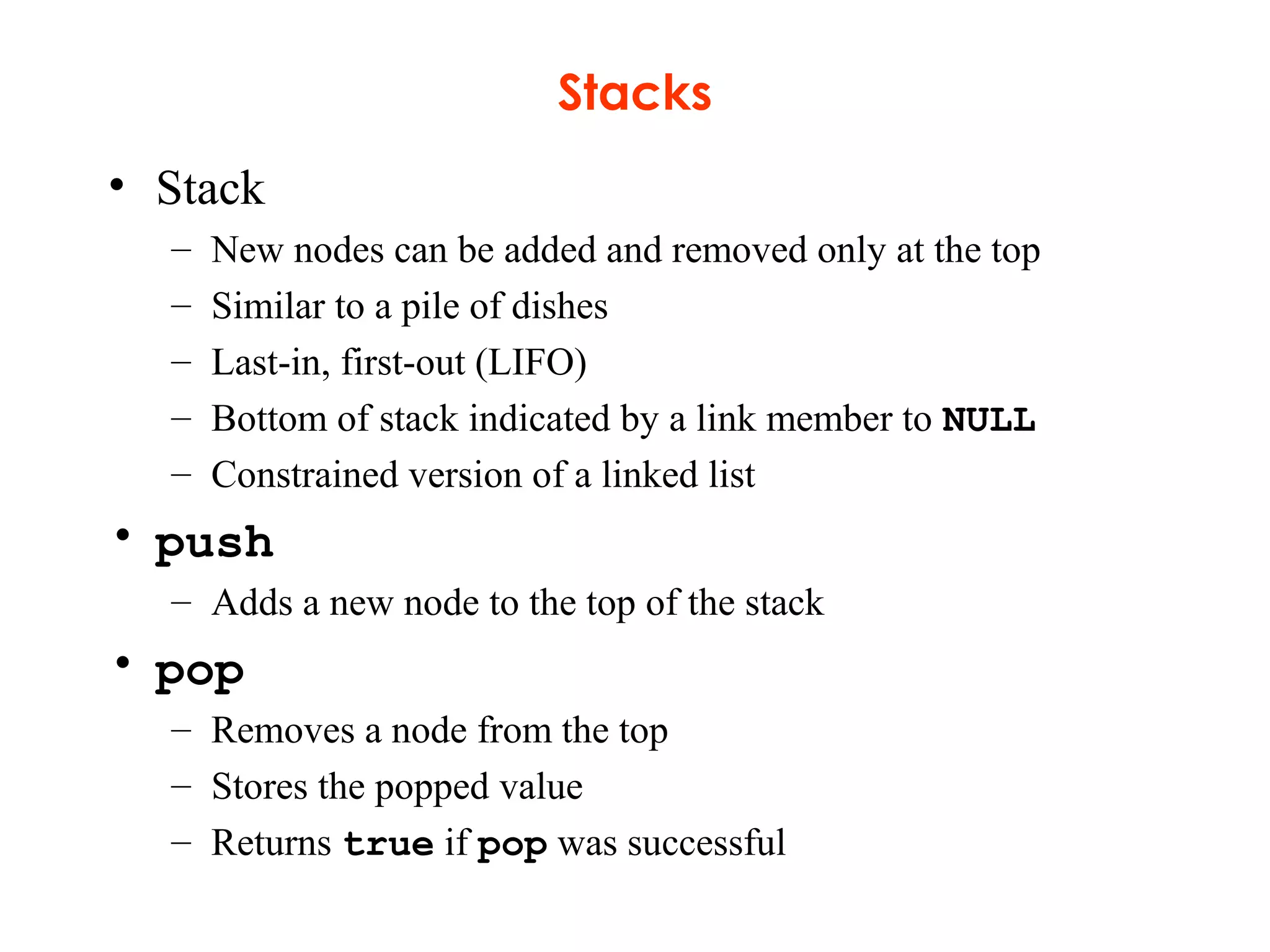
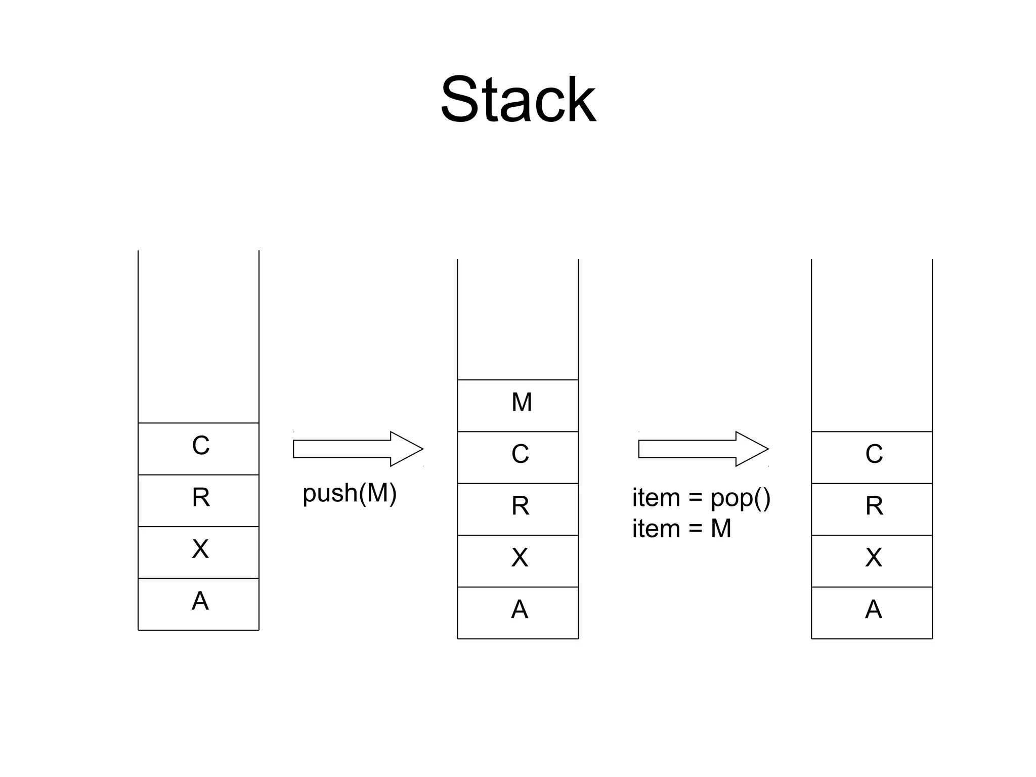
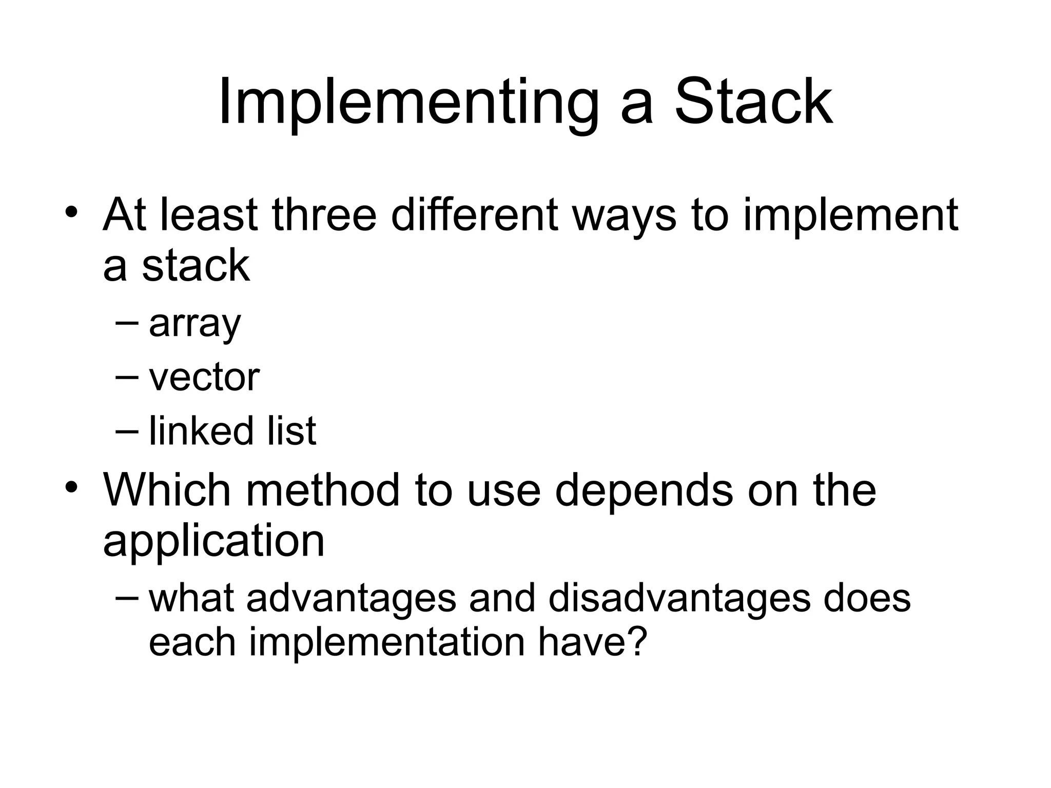
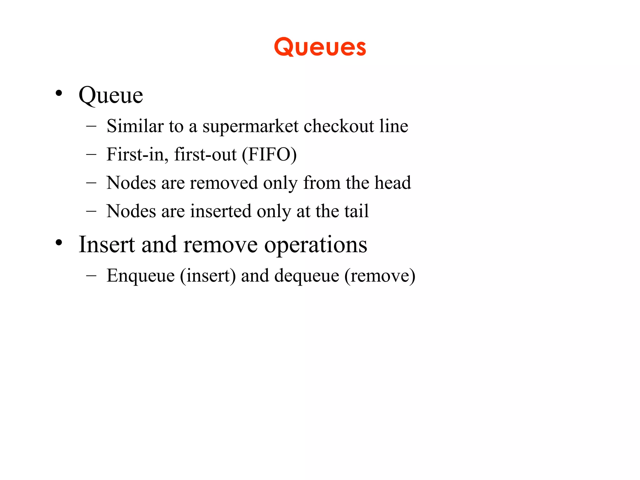
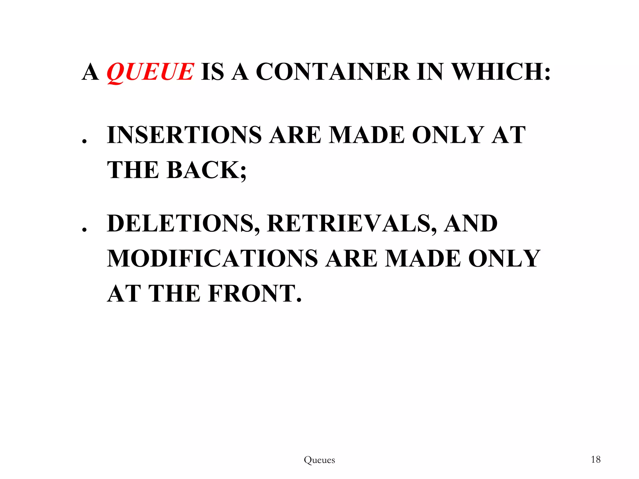
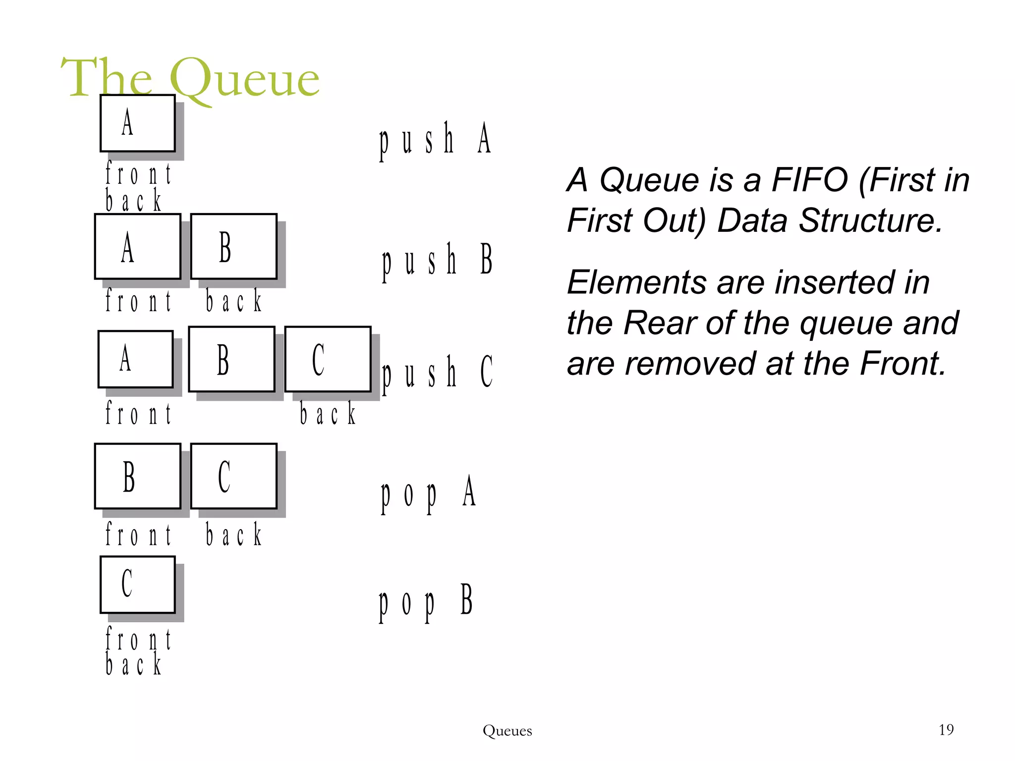
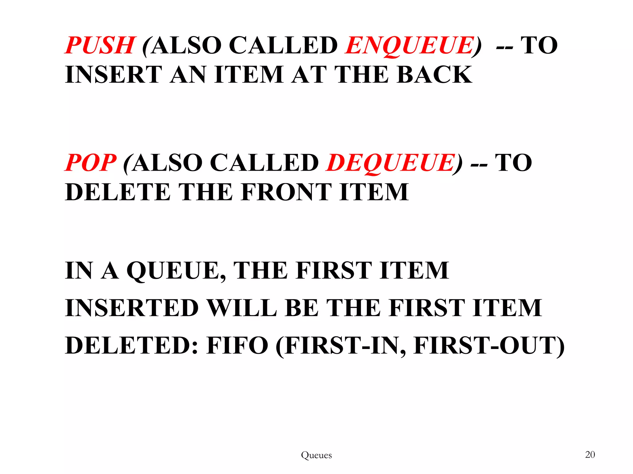
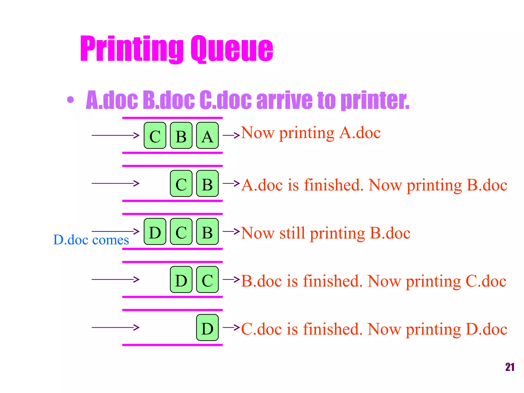
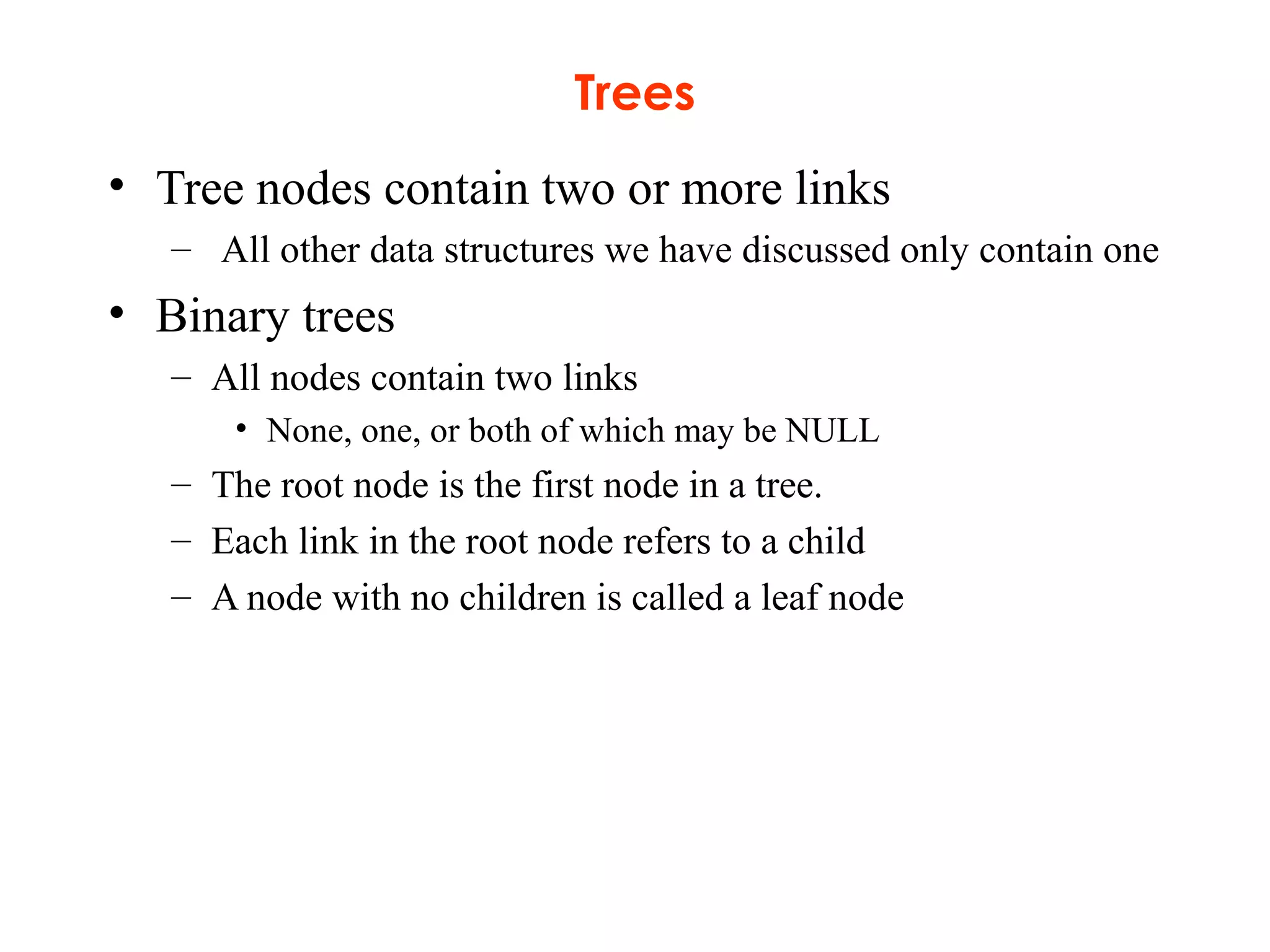
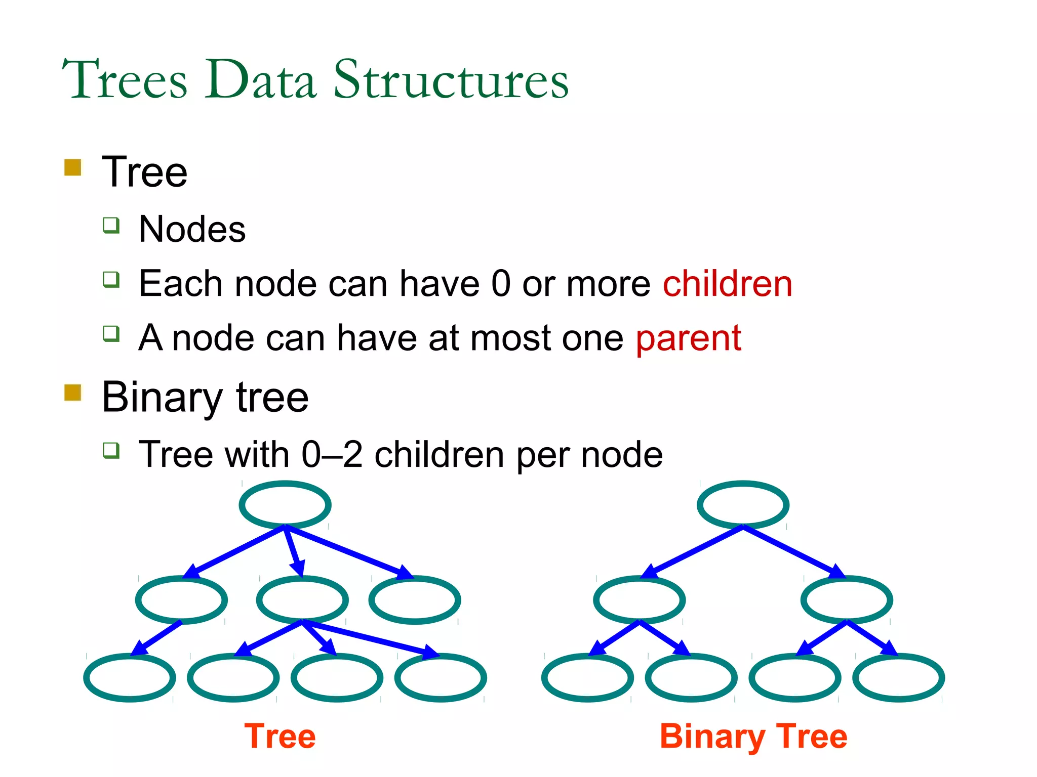
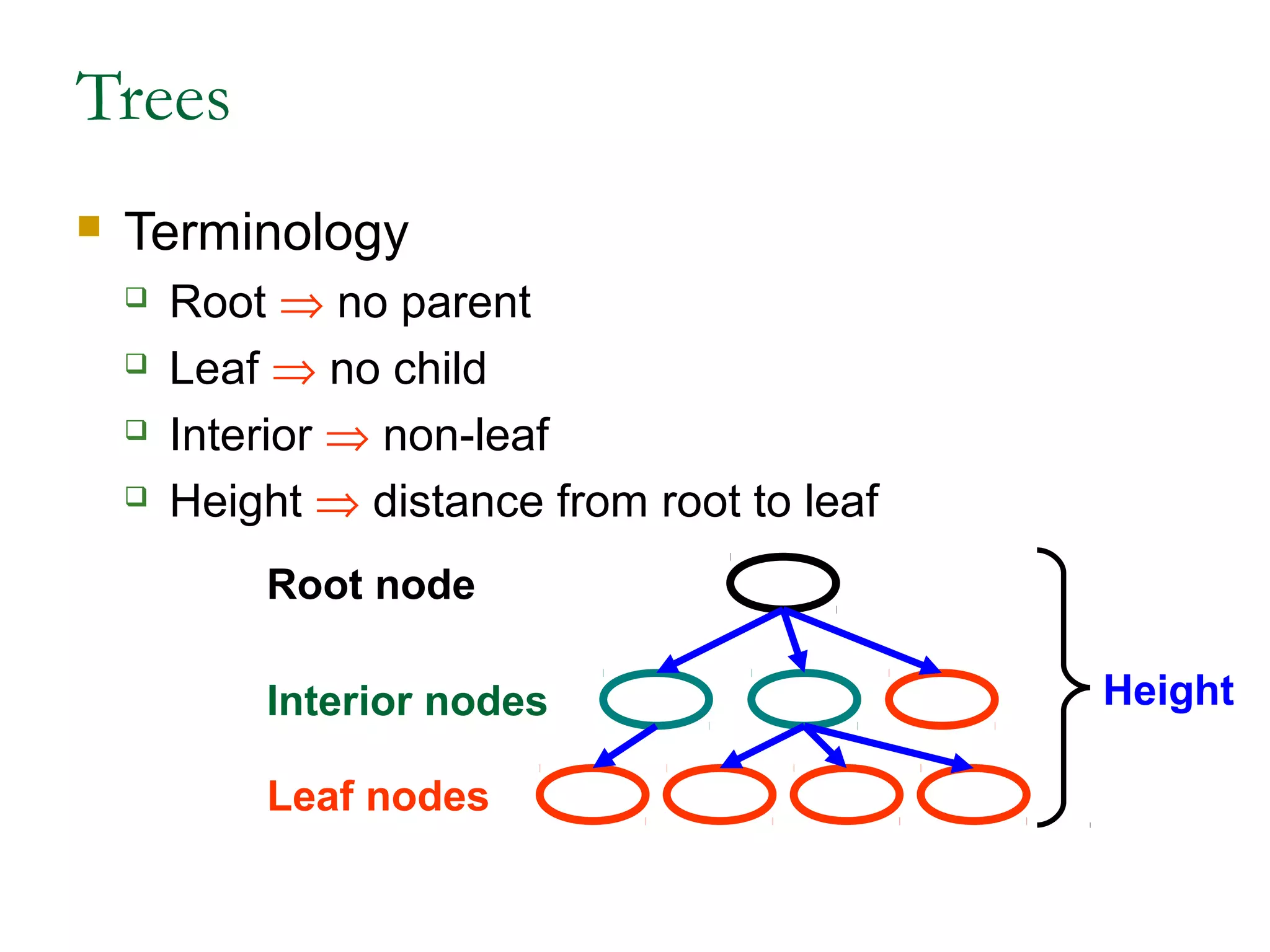
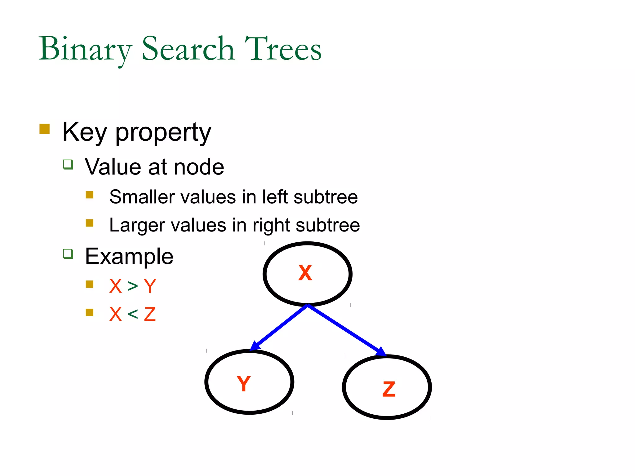
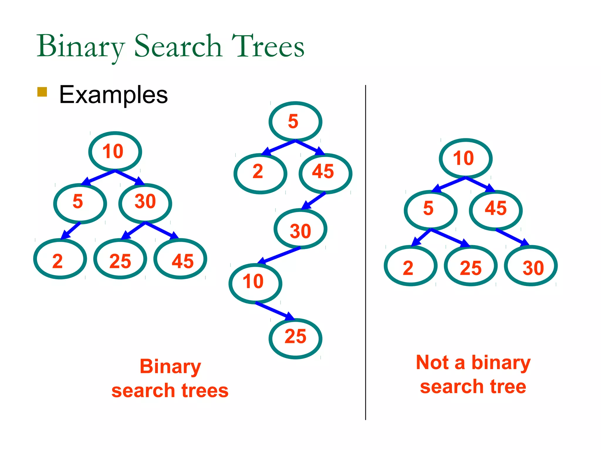
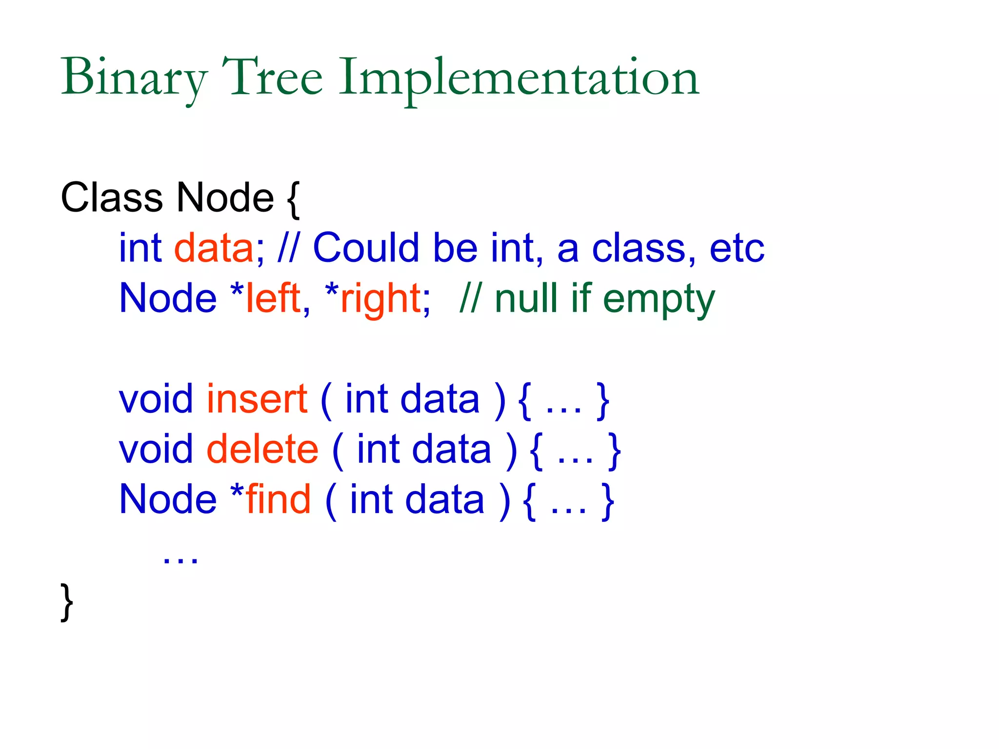
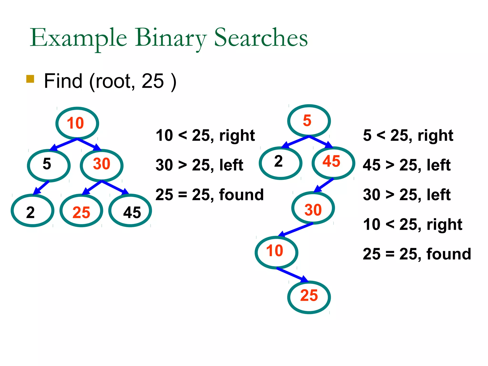
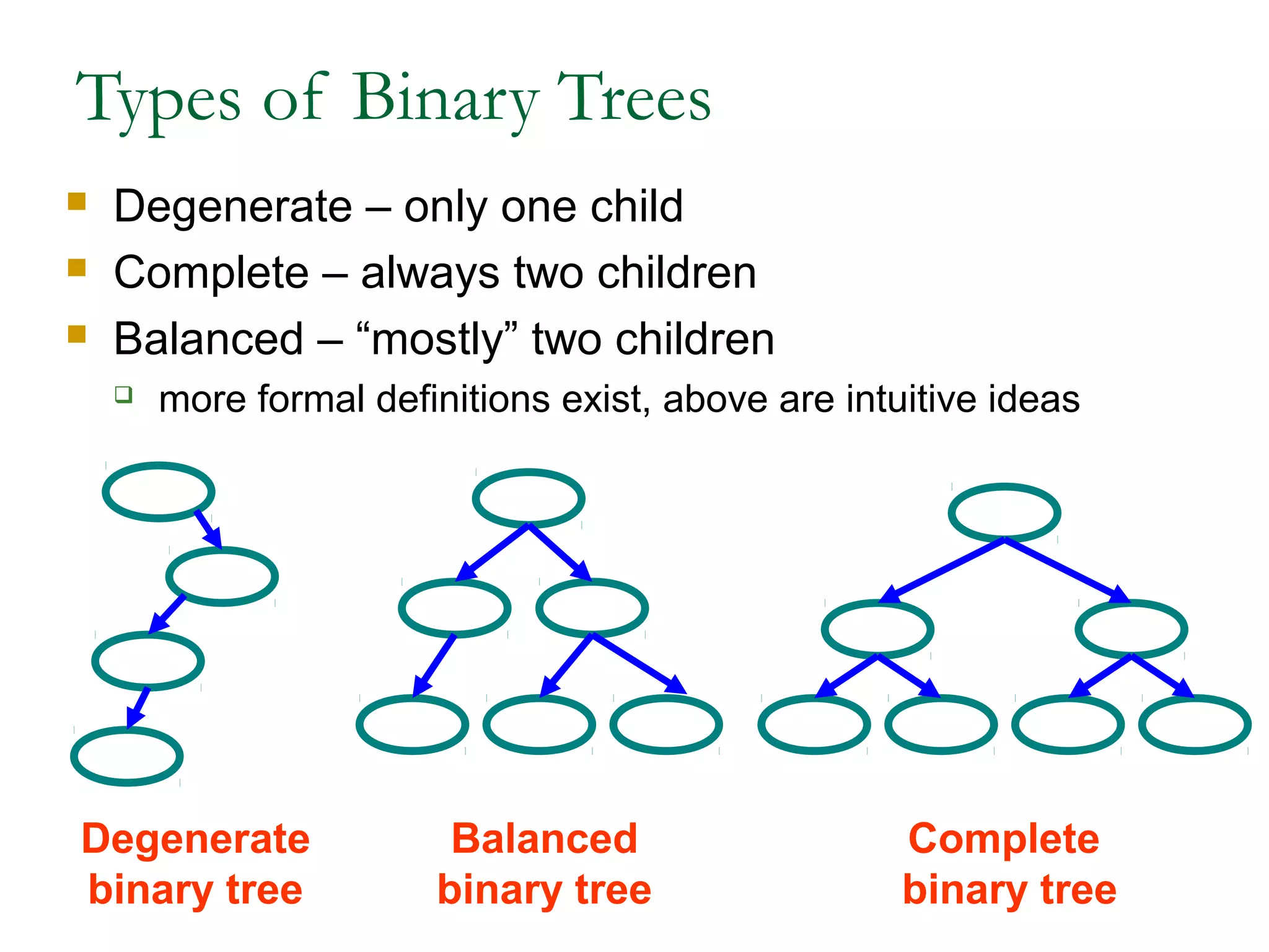
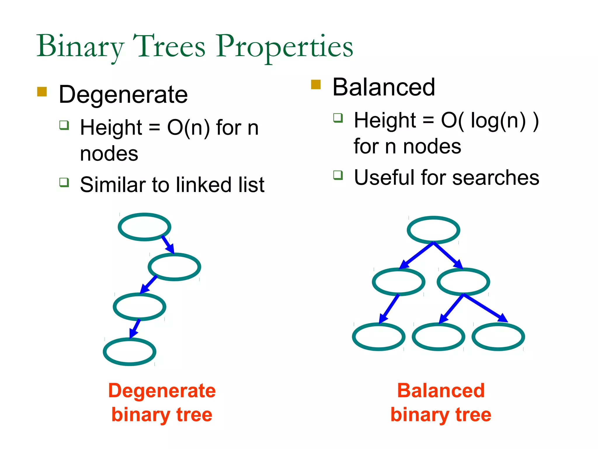
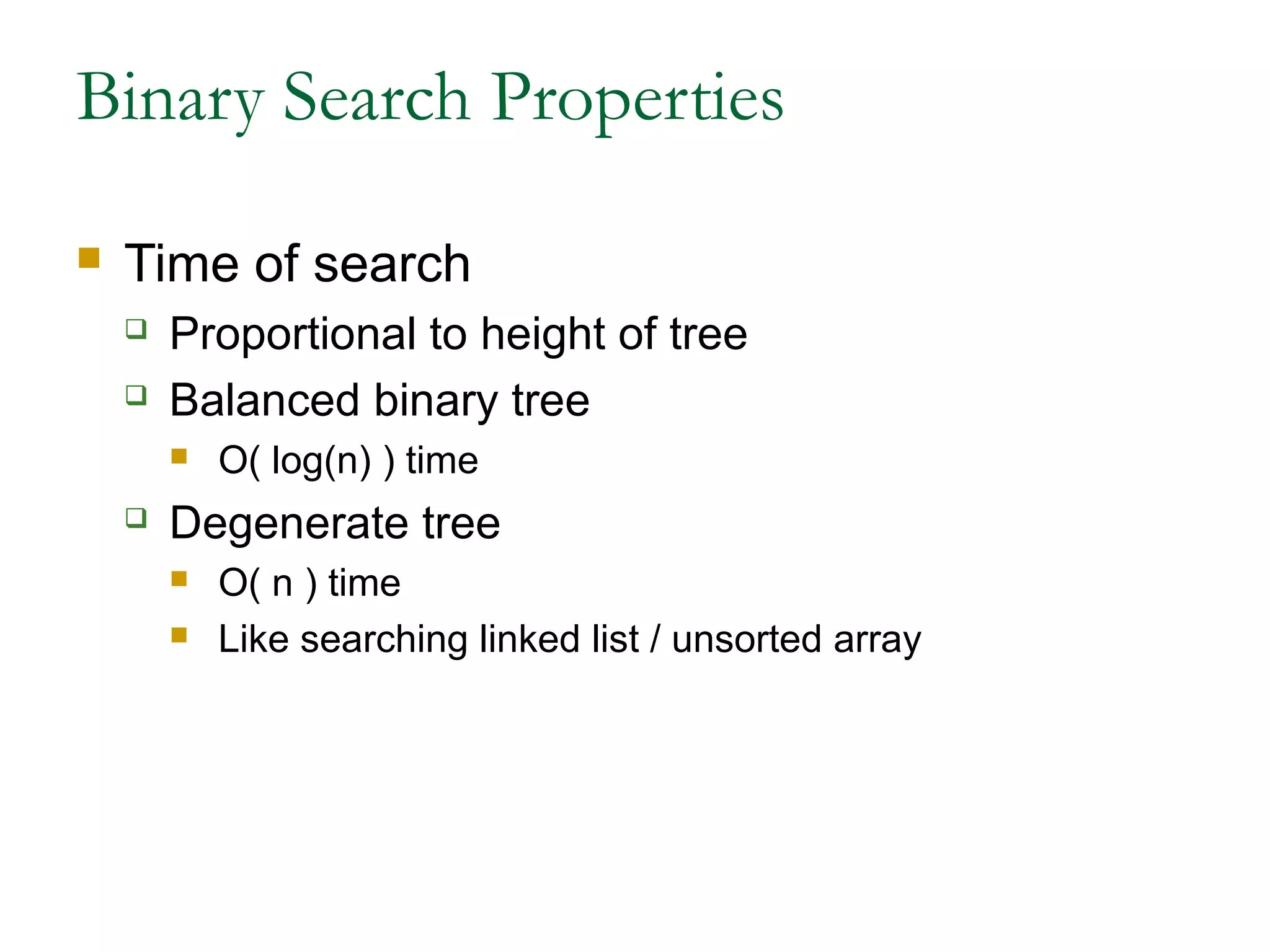
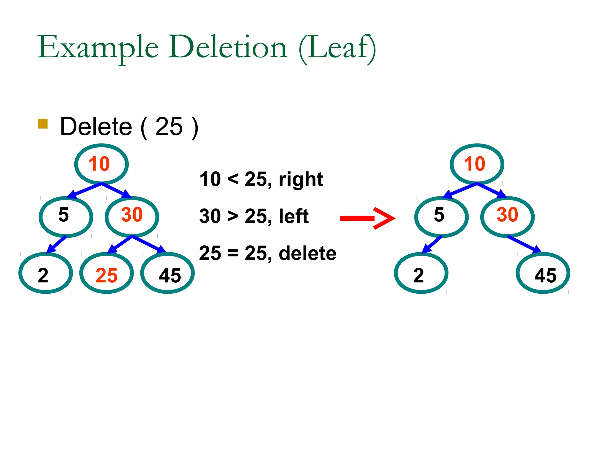
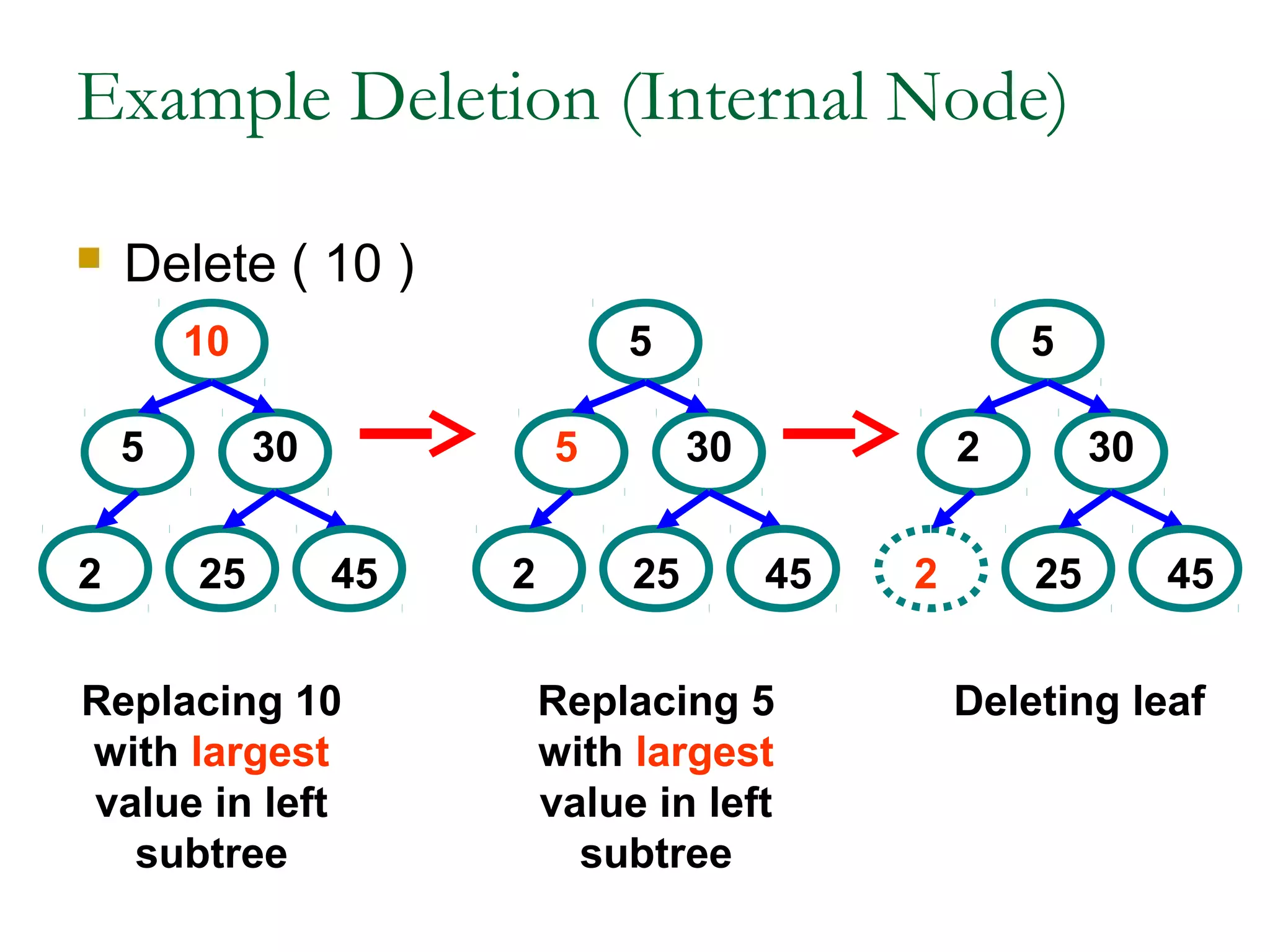
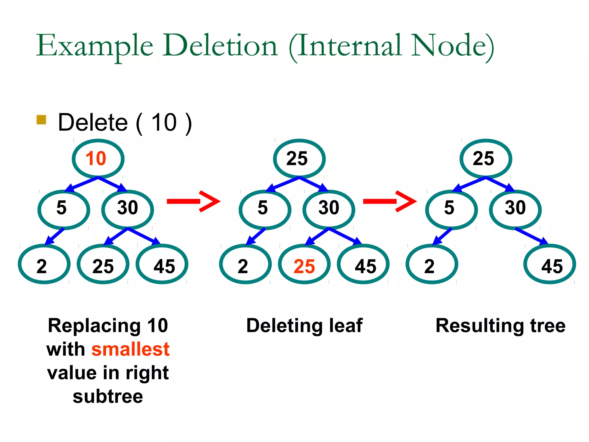
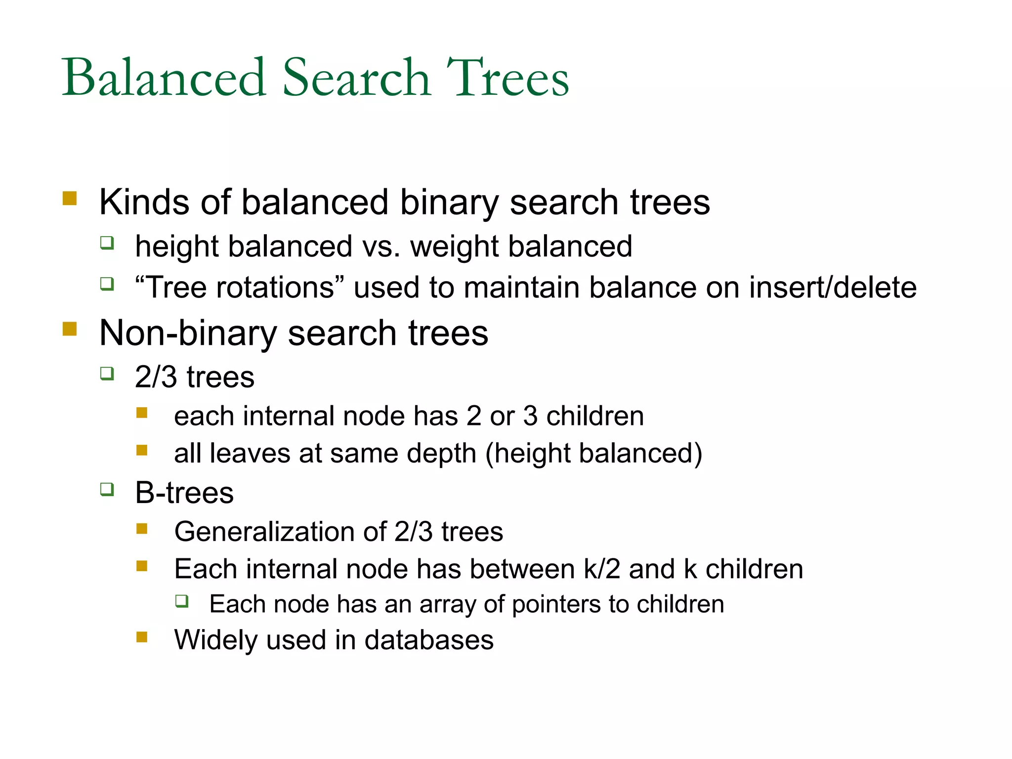
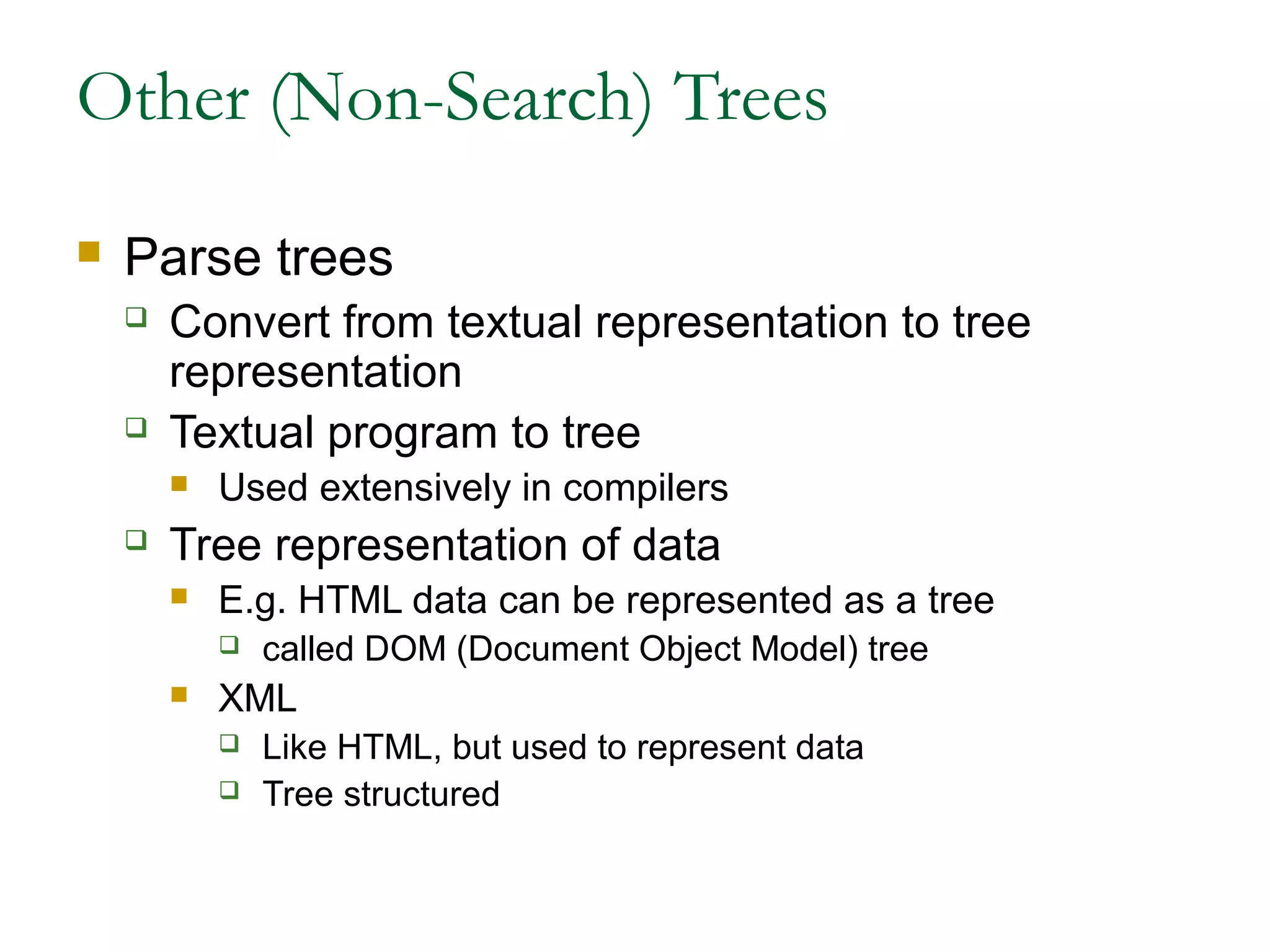
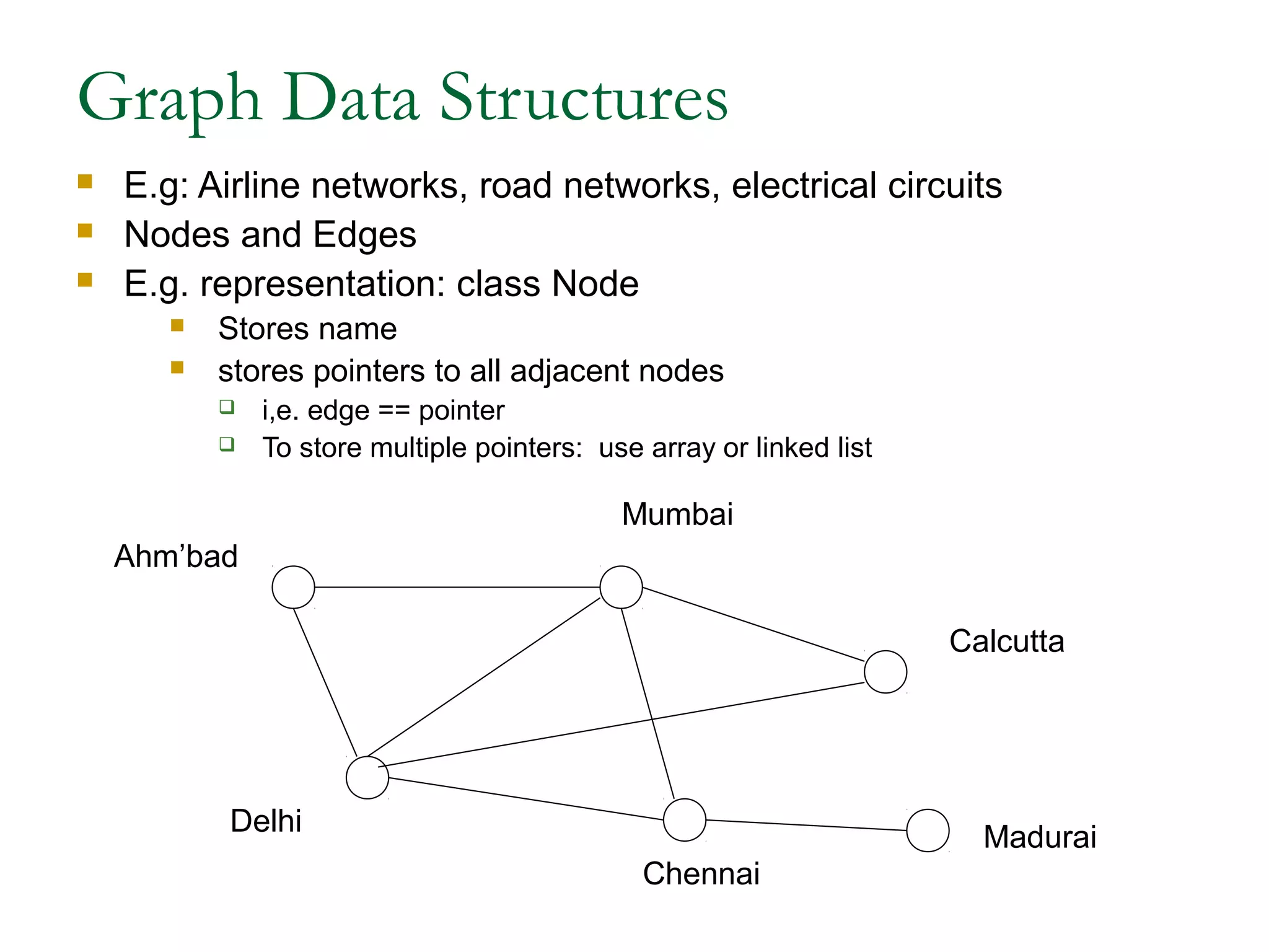

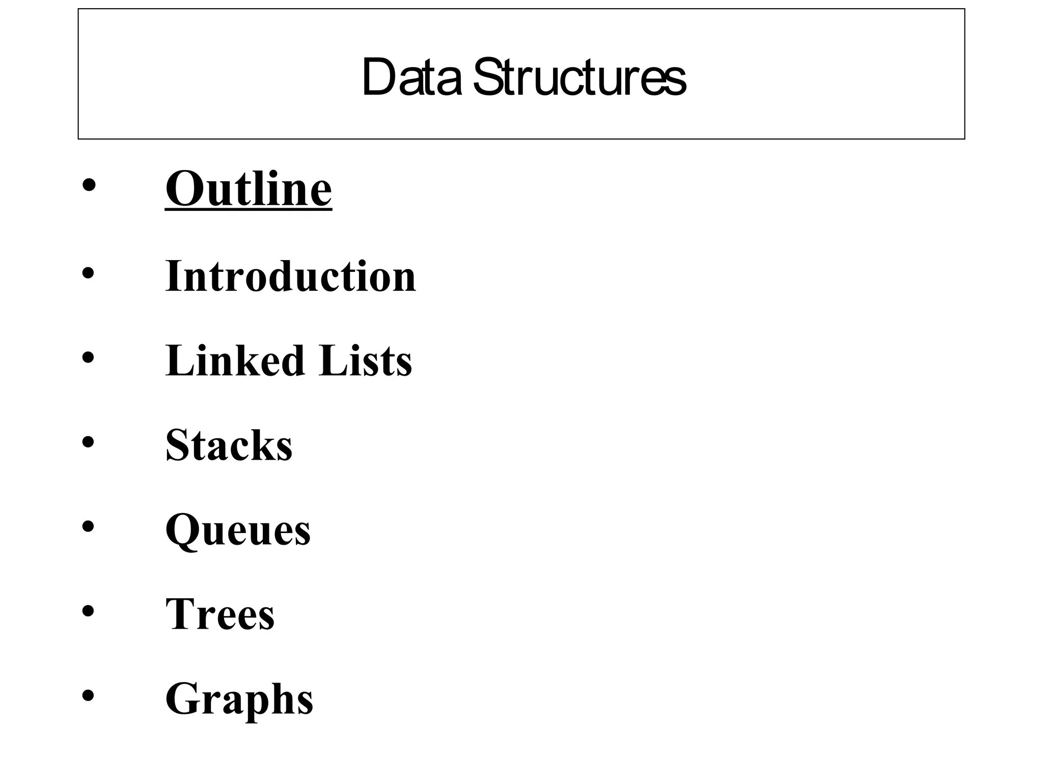
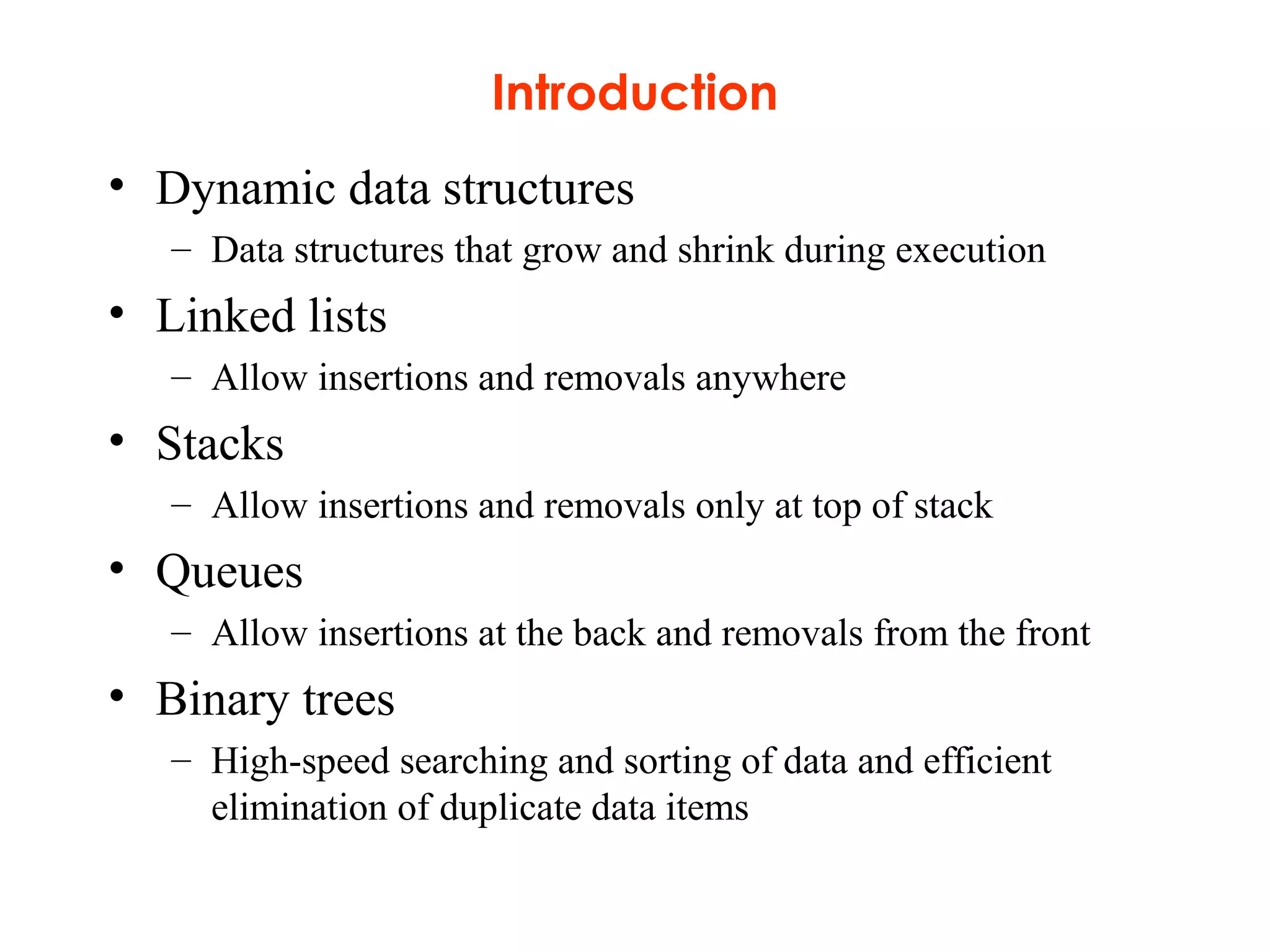
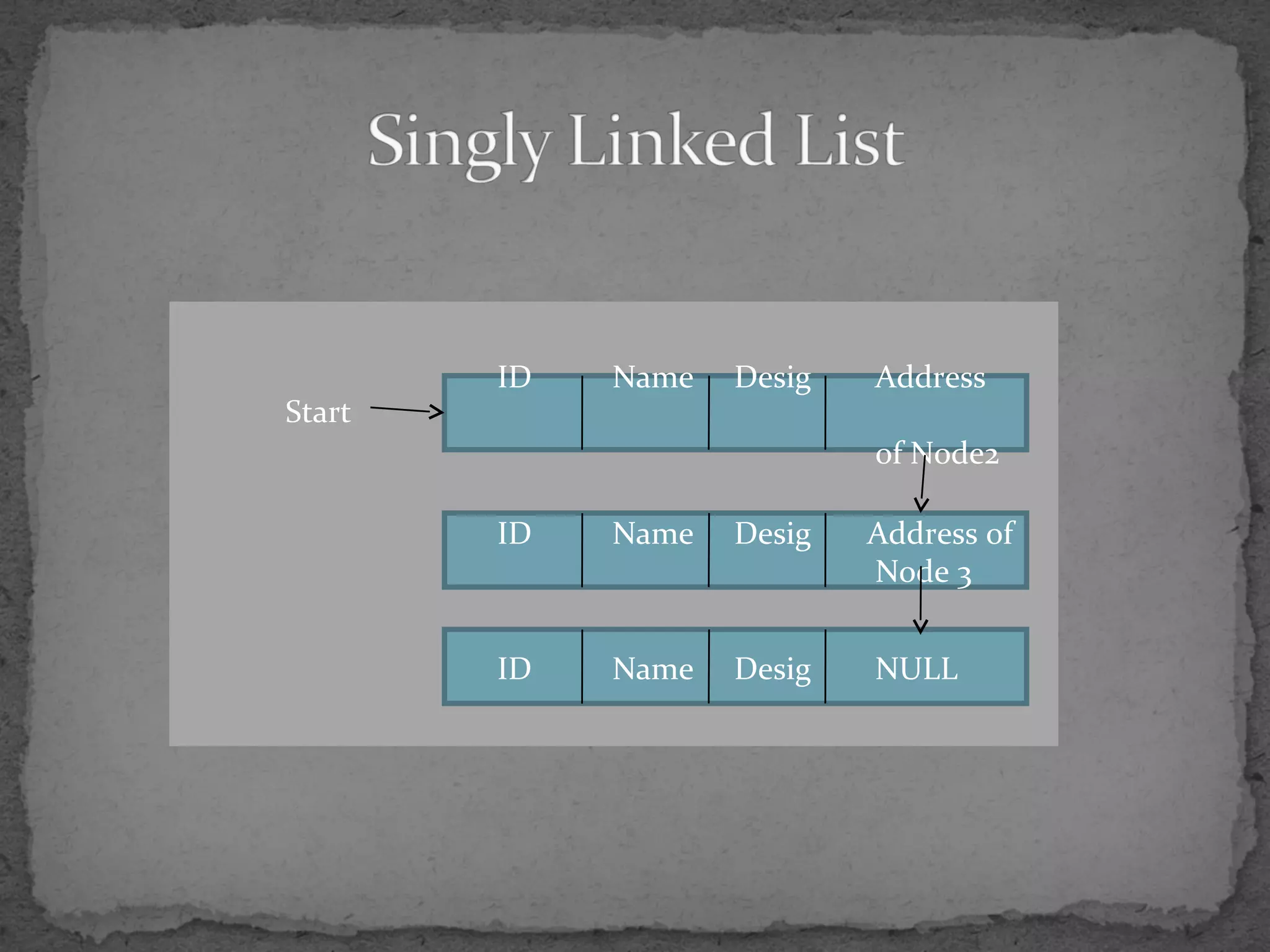
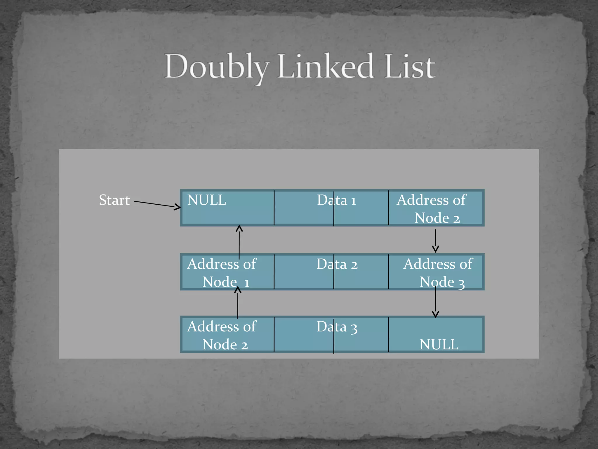
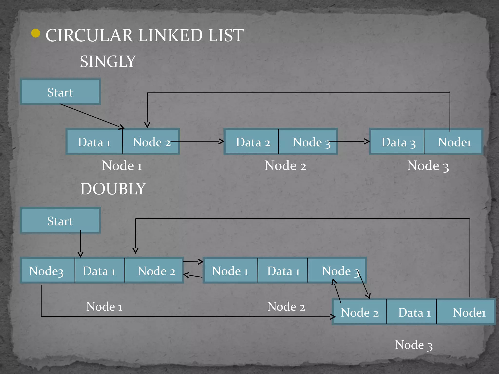
This document provides an introduction and overview of common data structures including linked lists, stacks, queues, trees, and graphs. It defines each structure and describes their basic operations and implementations. Linked lists allow insertions and deletions anywhere and come in singly and doubly linked varieties. Stacks and queues follow last-in, first-out and first-in, first-out rules respectively. Binary trees enable fast searching and sorting of data. Graphs represent relationships between nodes connected by edges.


![[Queue , linked list , tree]](https://cdn.slidesharecdn.com/ss_thumbnails/queuelinkedlisttree-200819083233-thumbnail.jpg?width=640&height=640&fit=bounds)