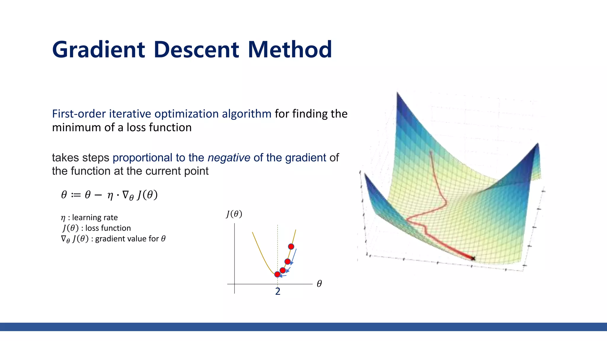
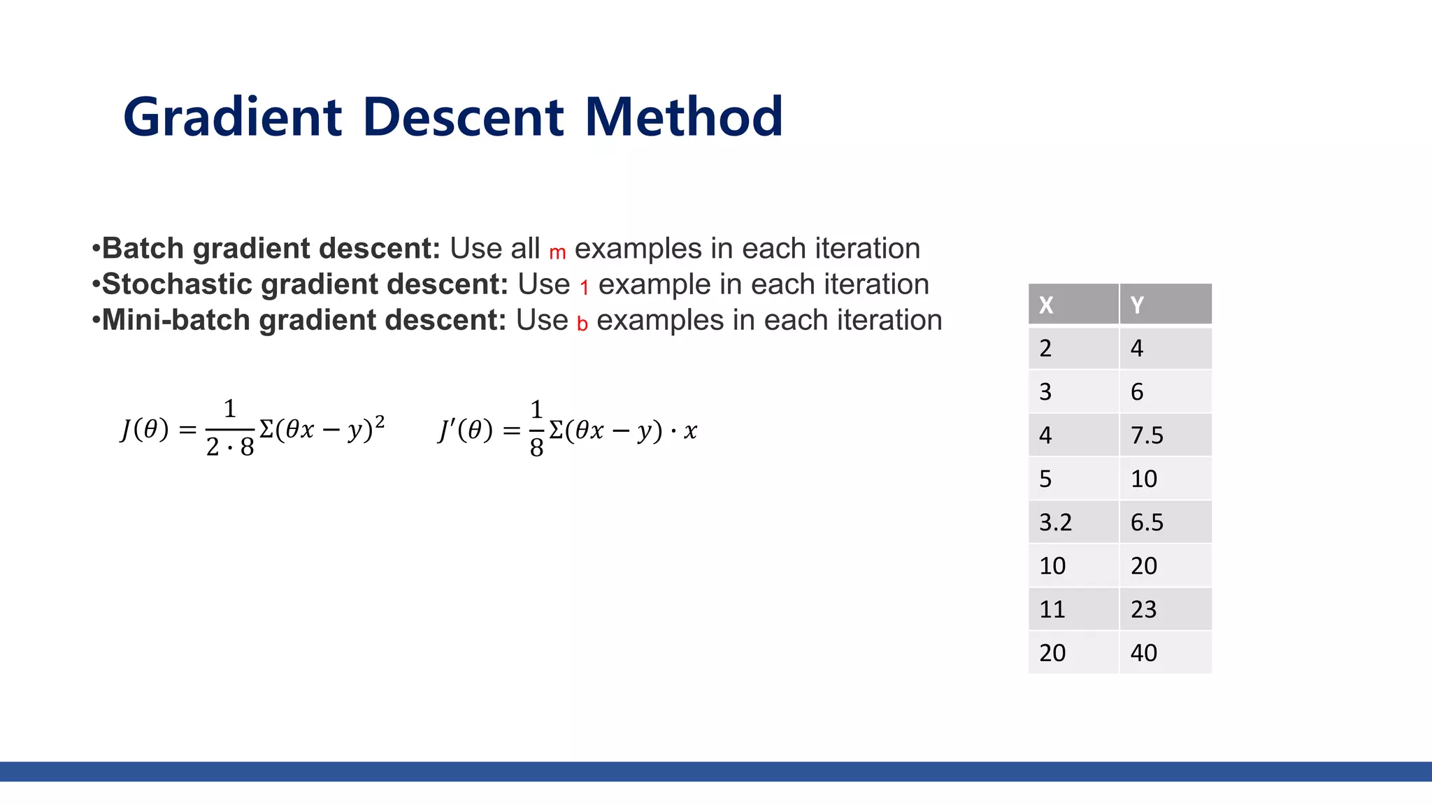
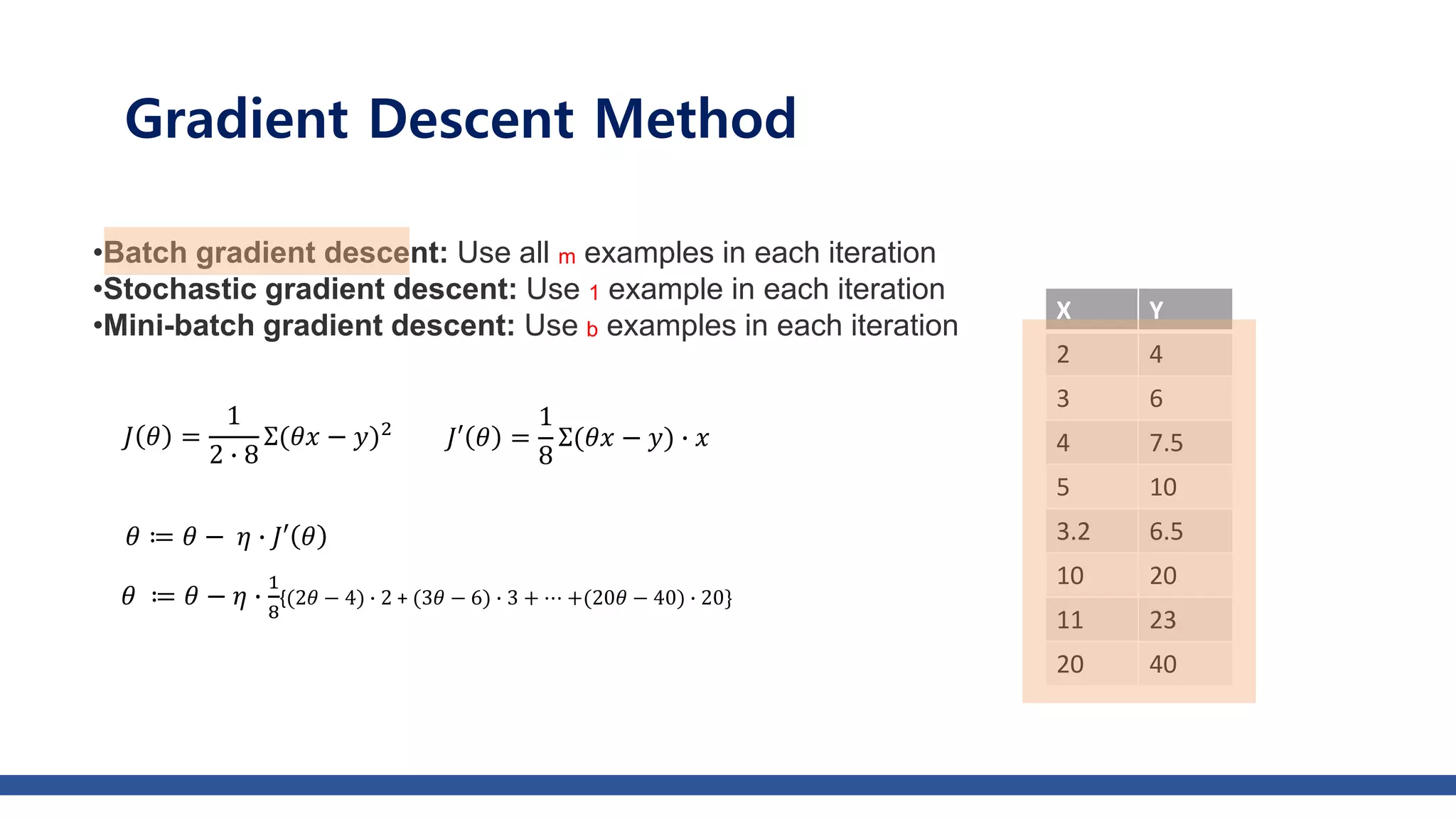
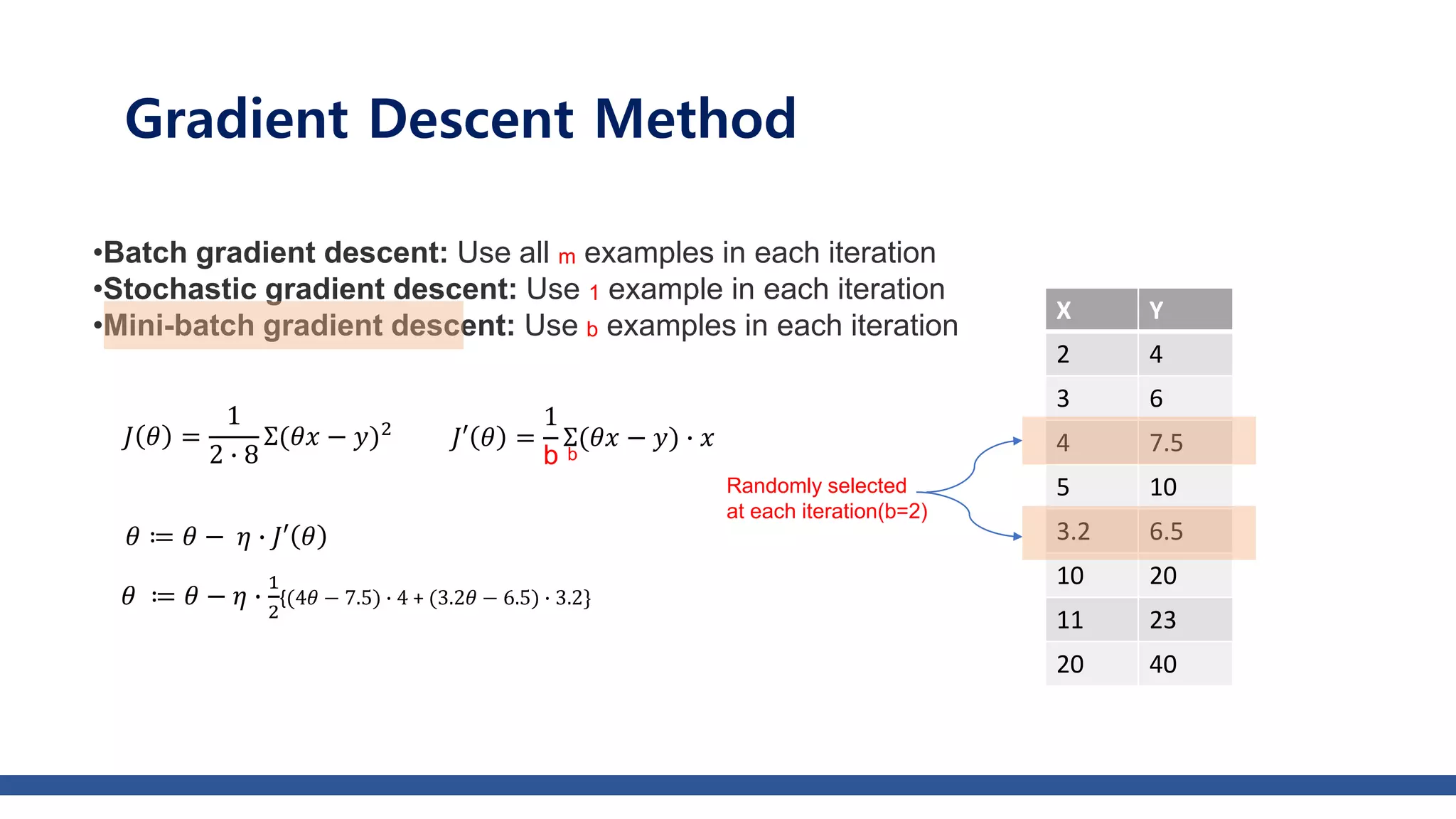
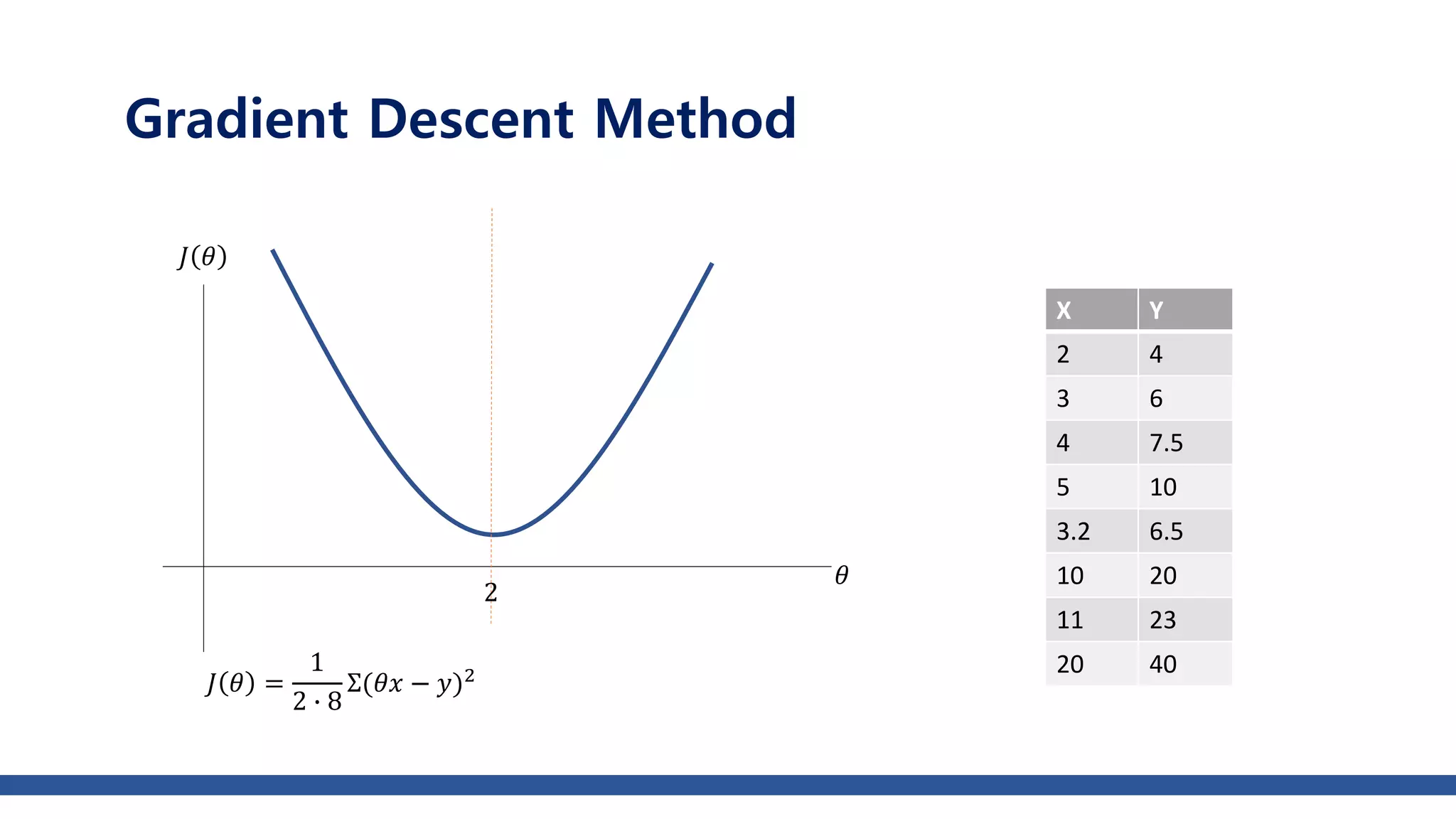
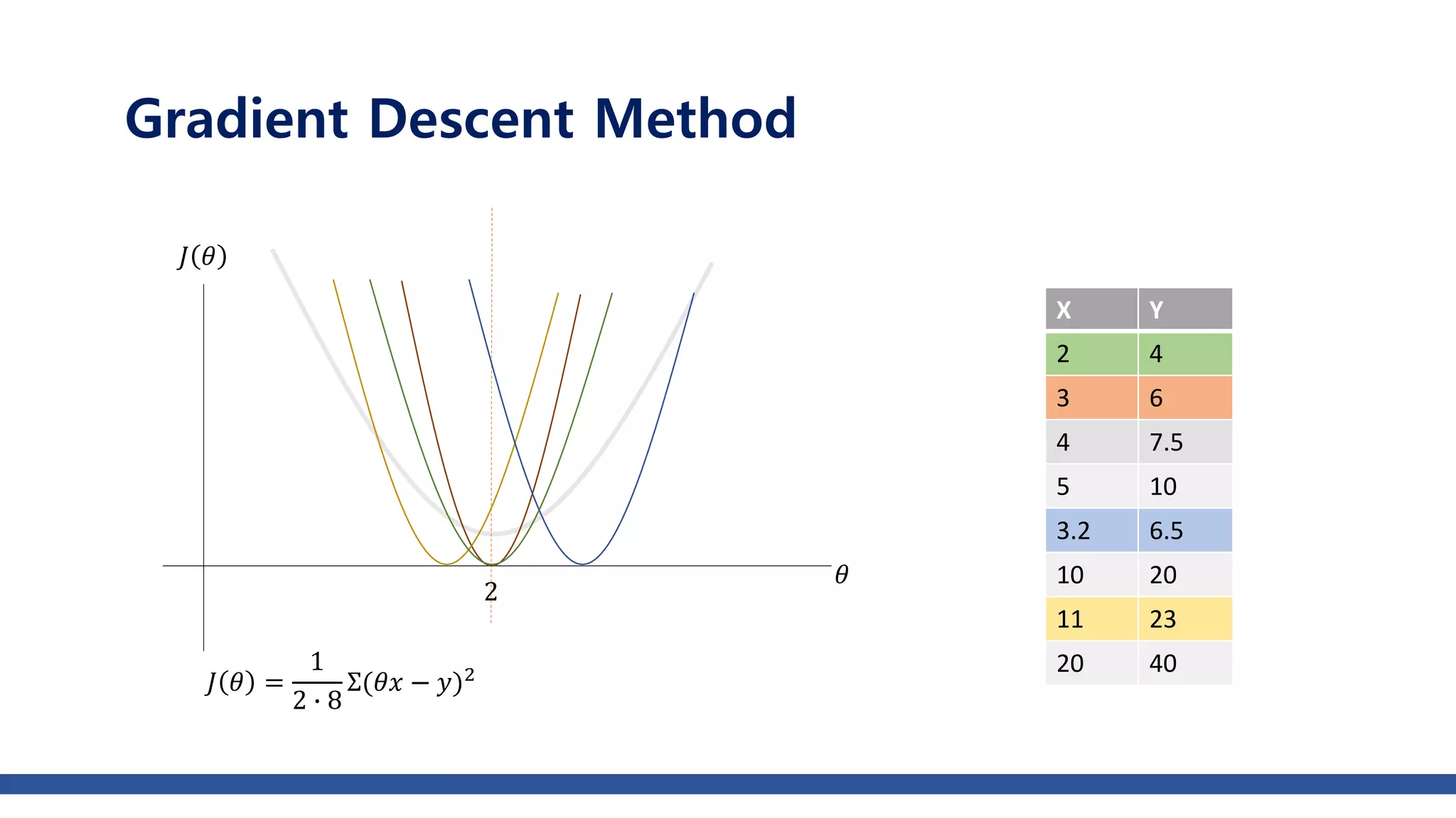
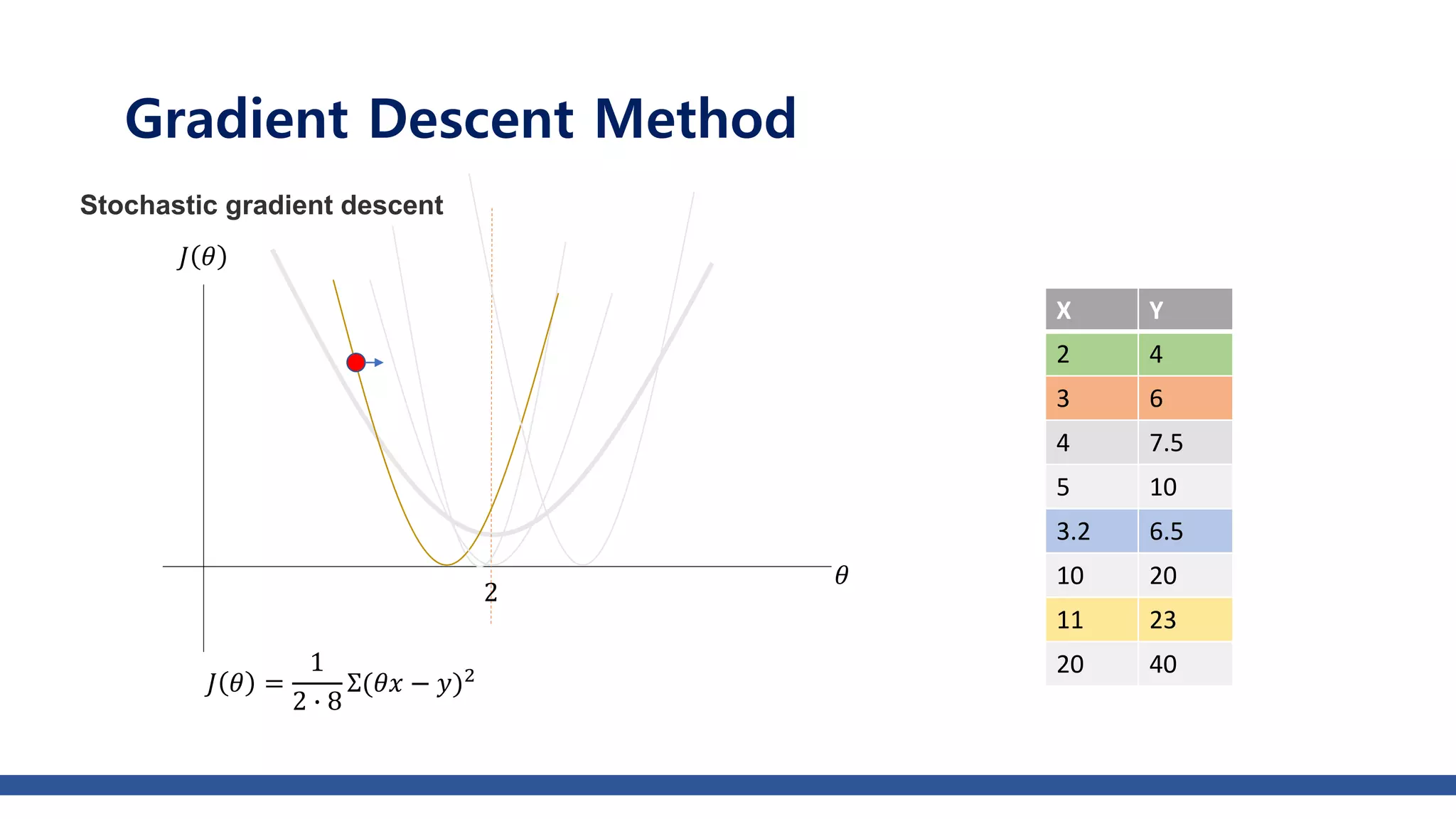
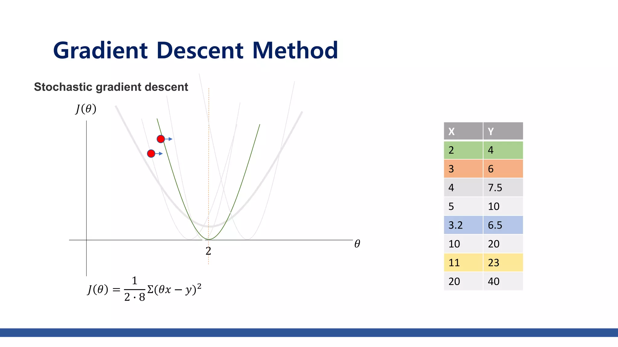
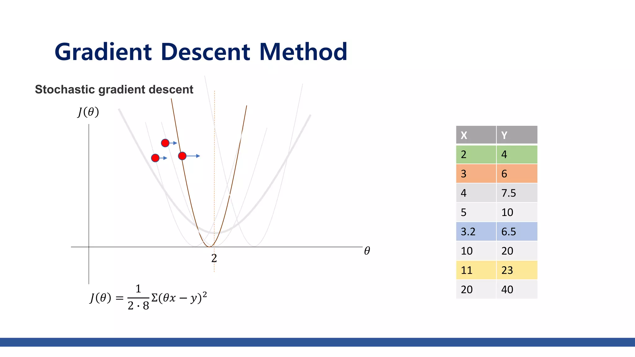
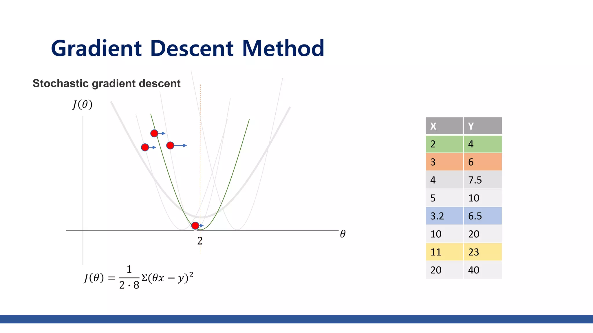
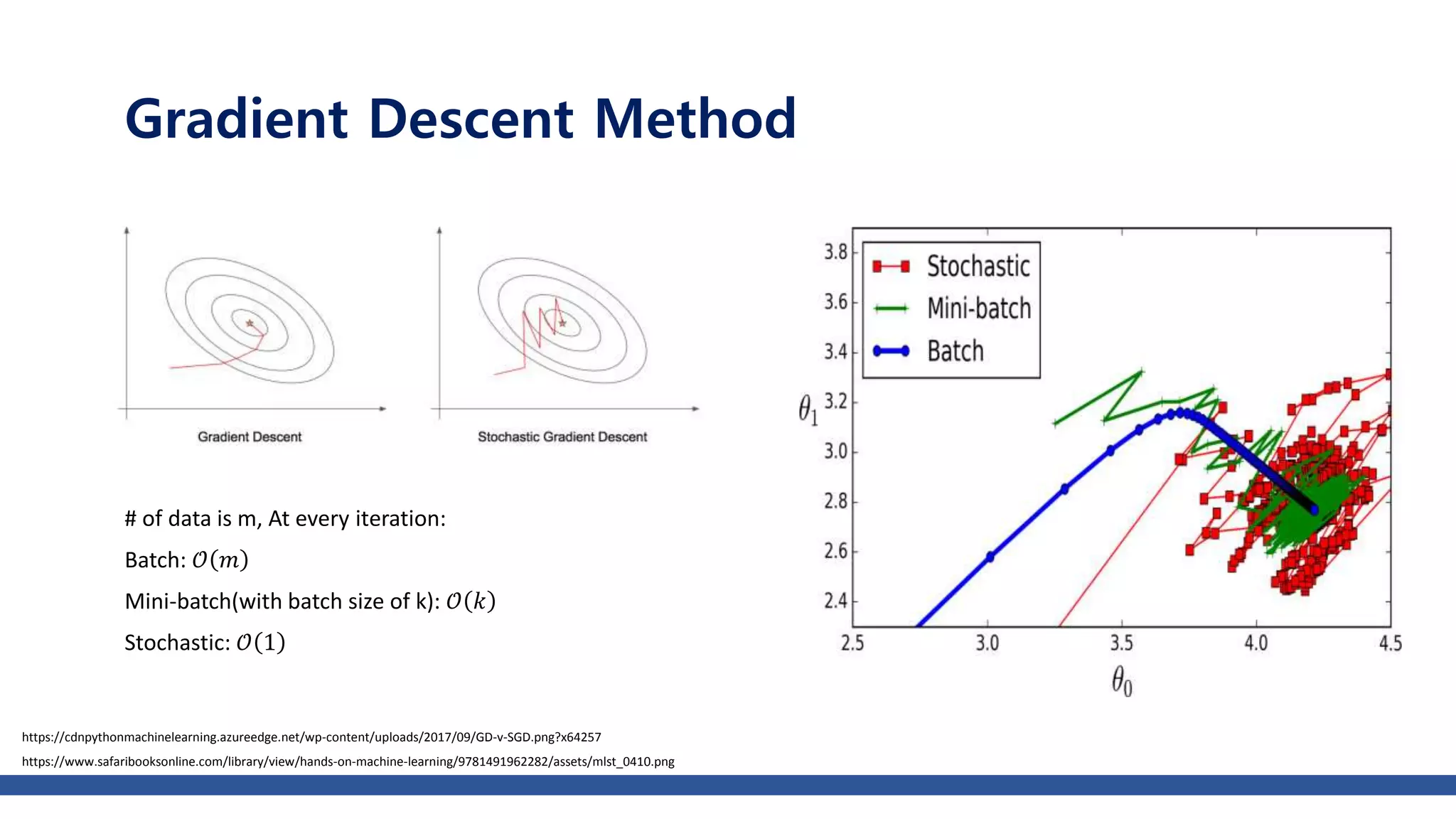
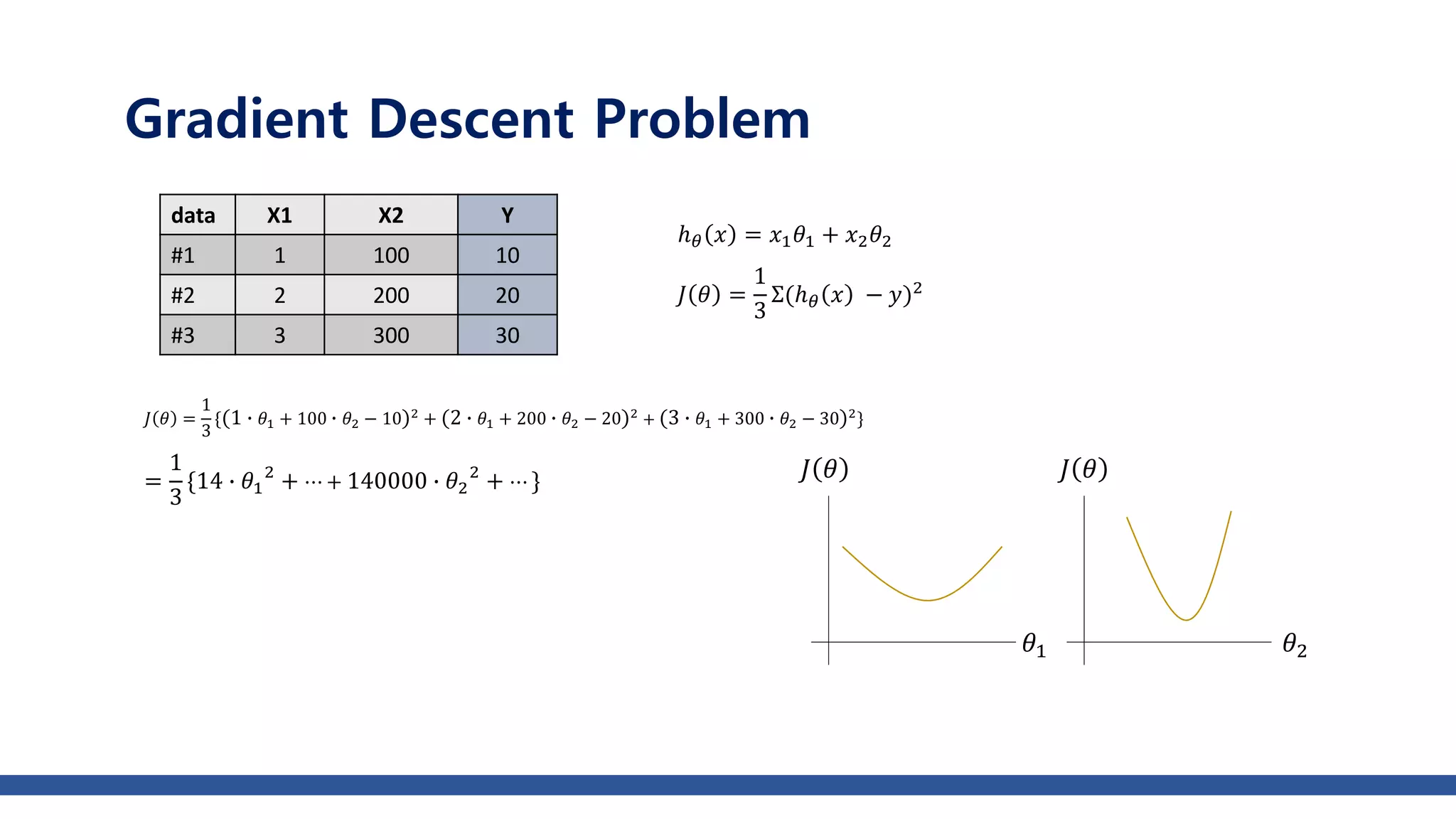
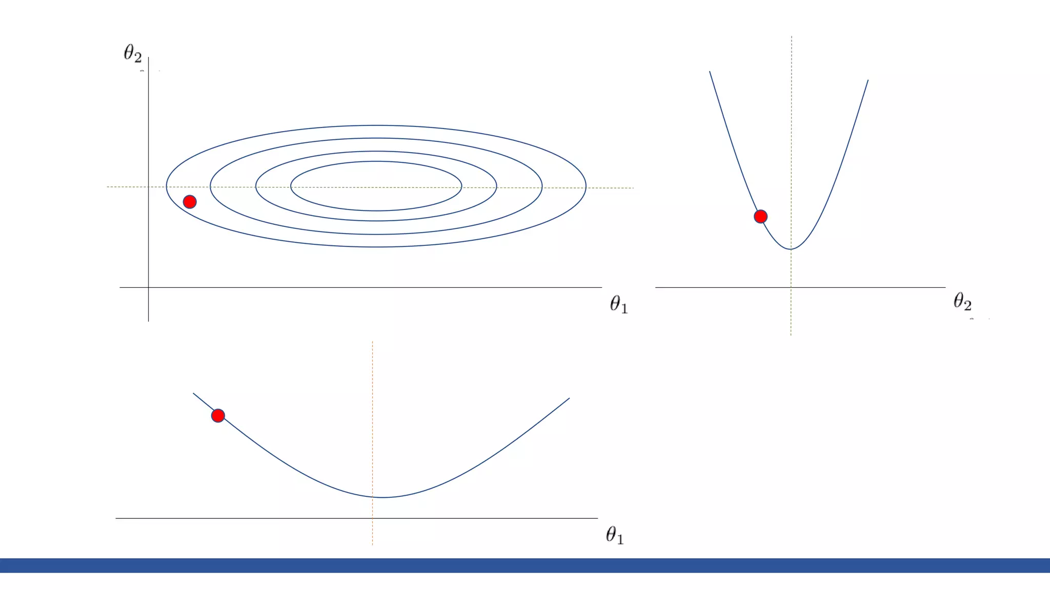
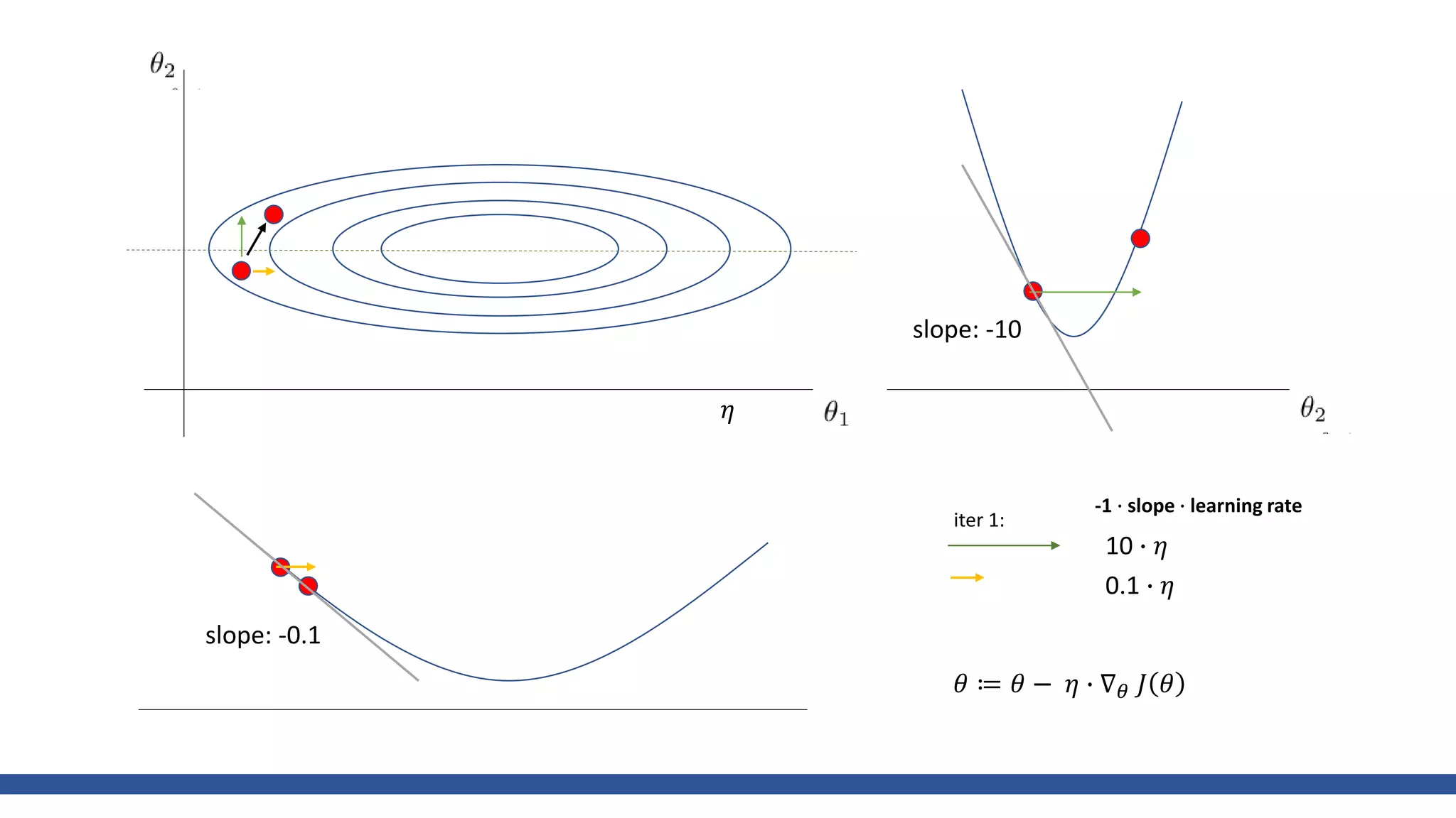
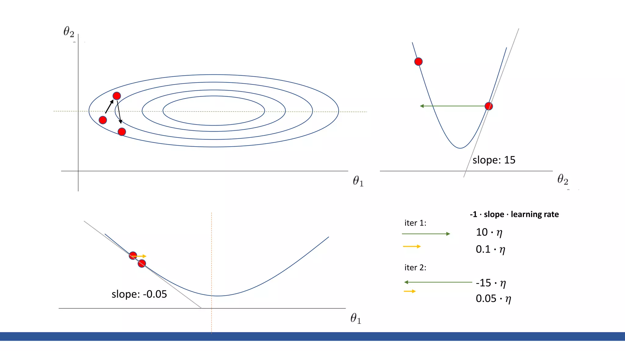
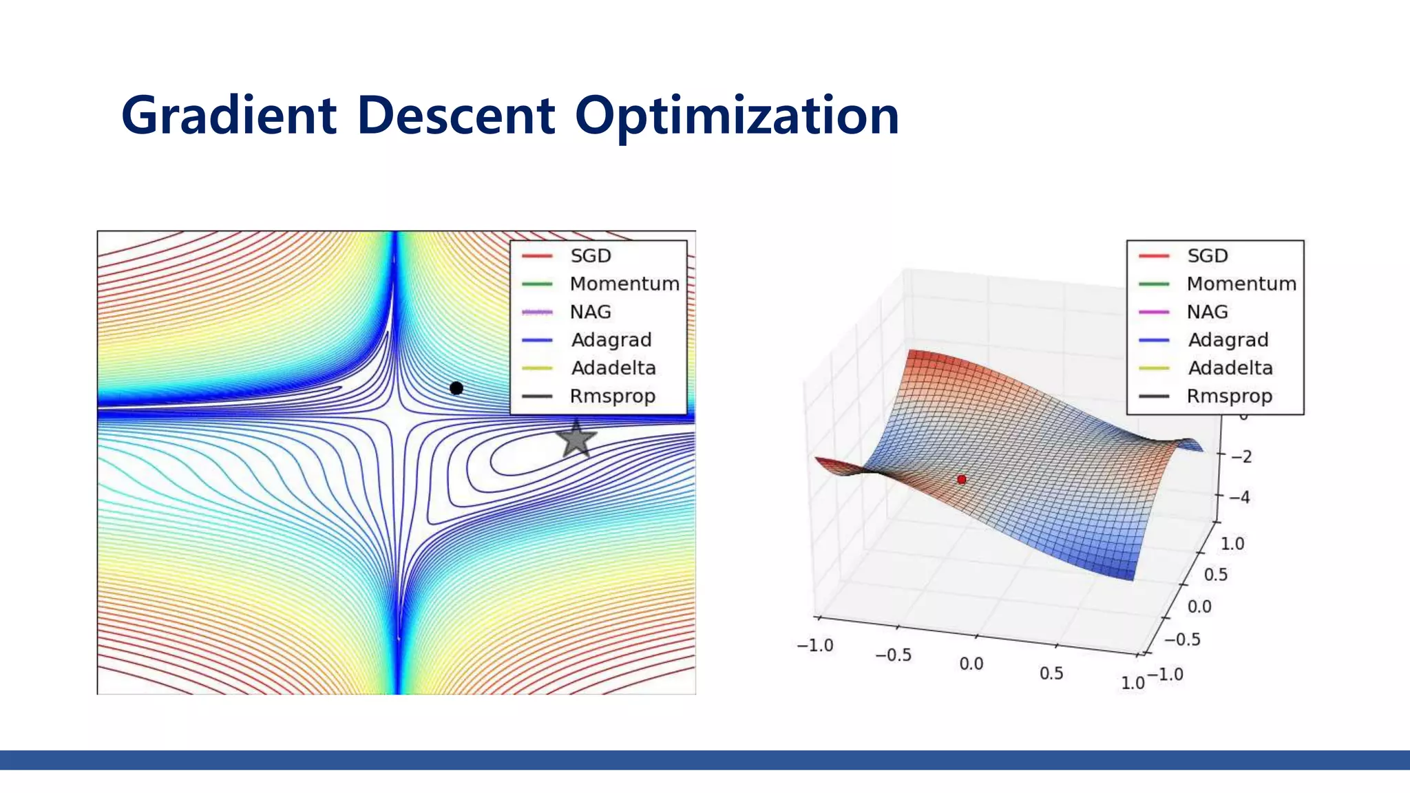
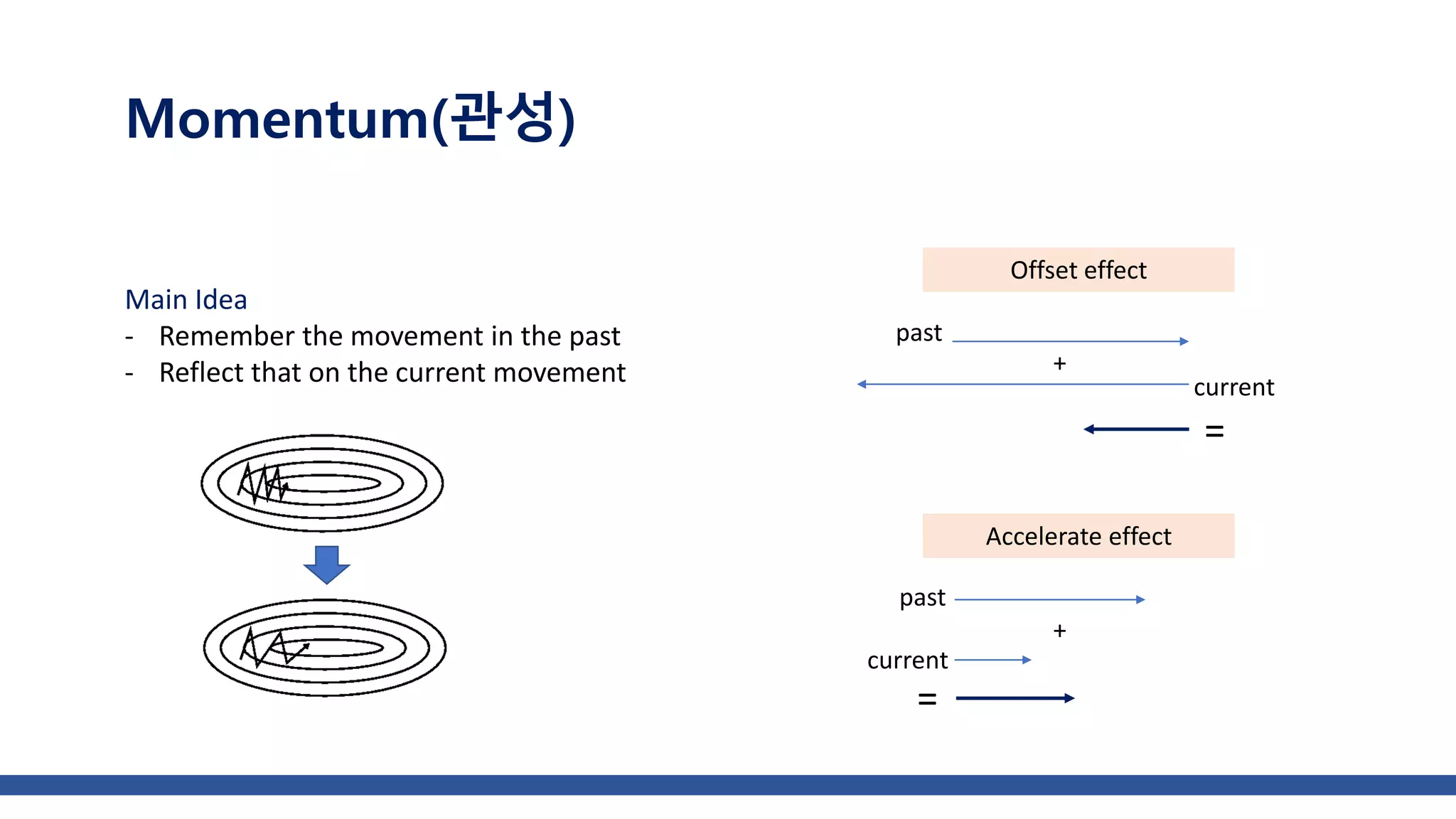
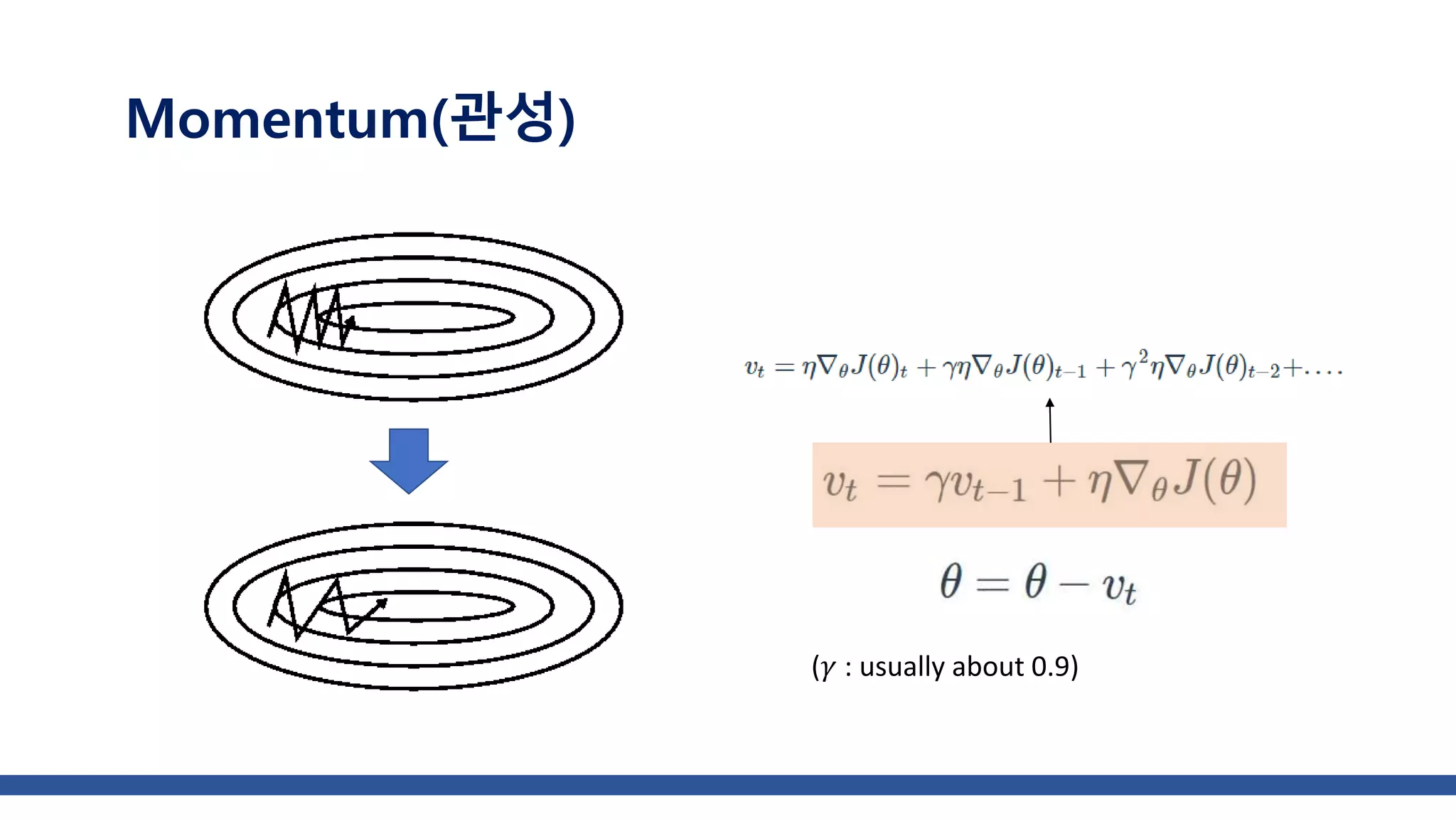
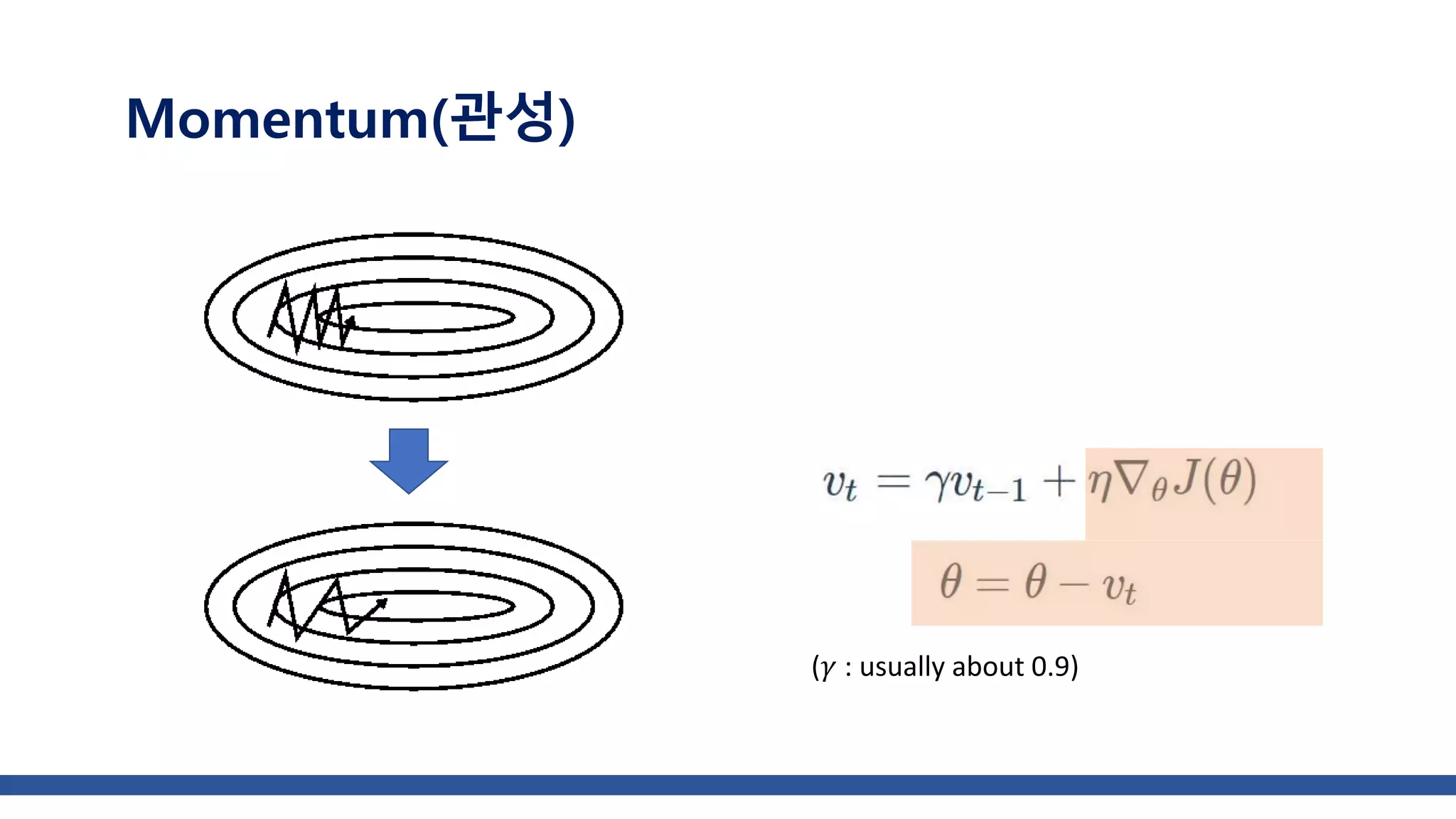
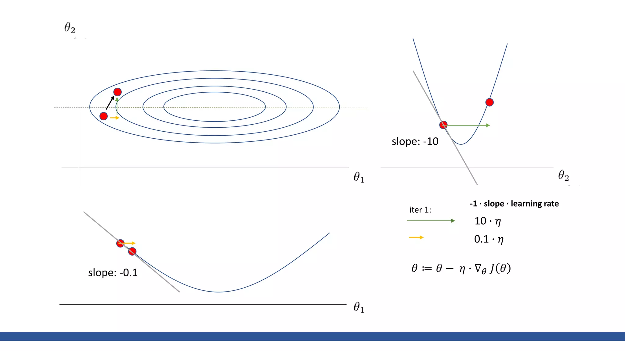
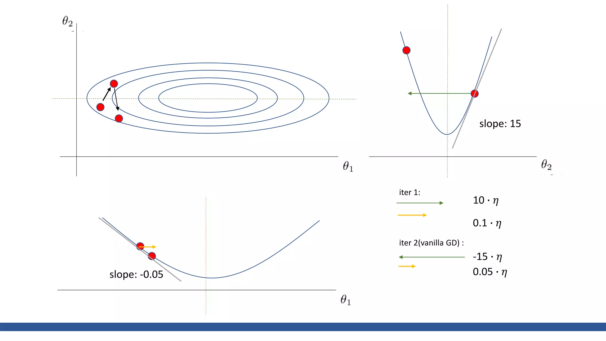
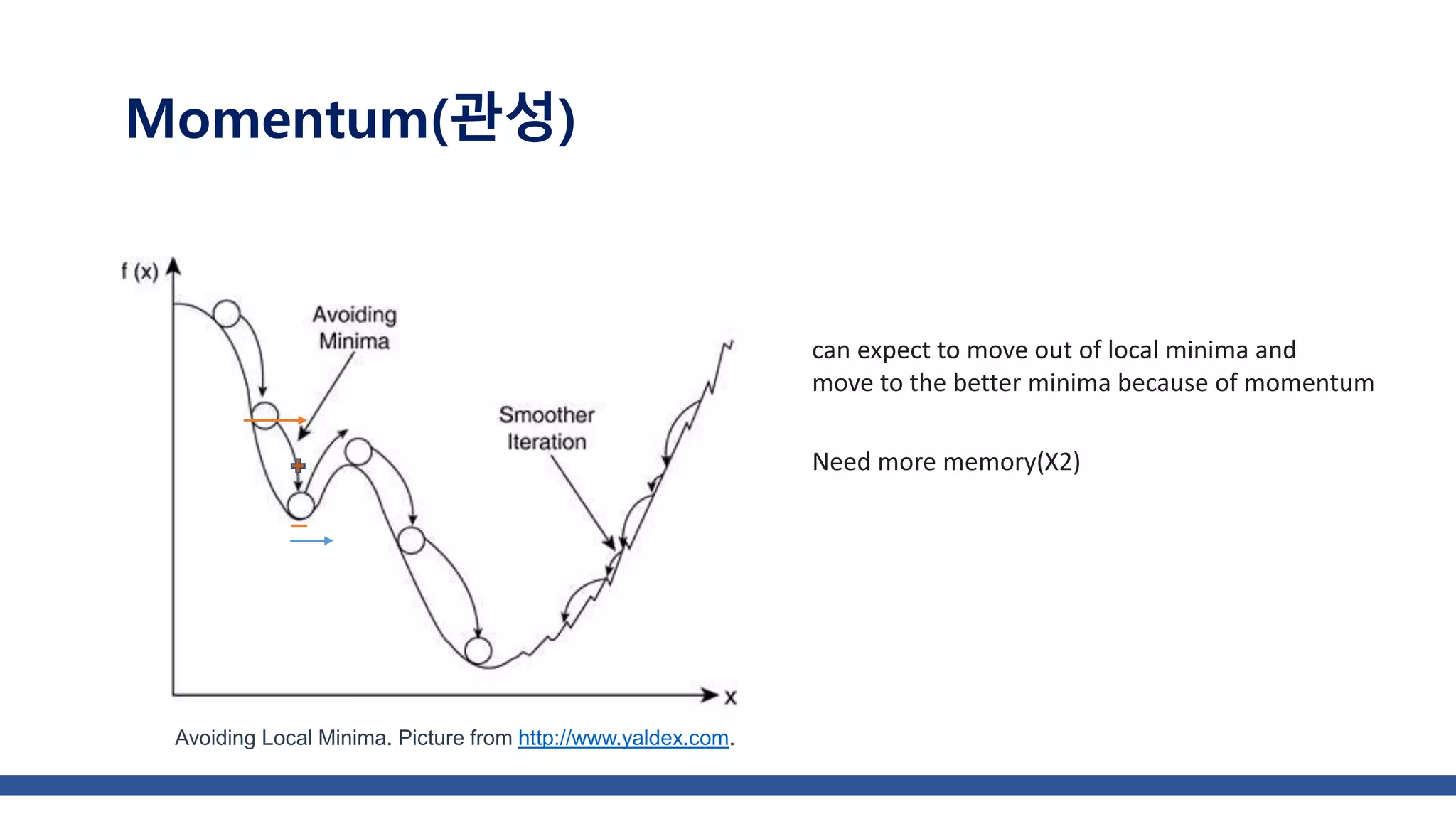
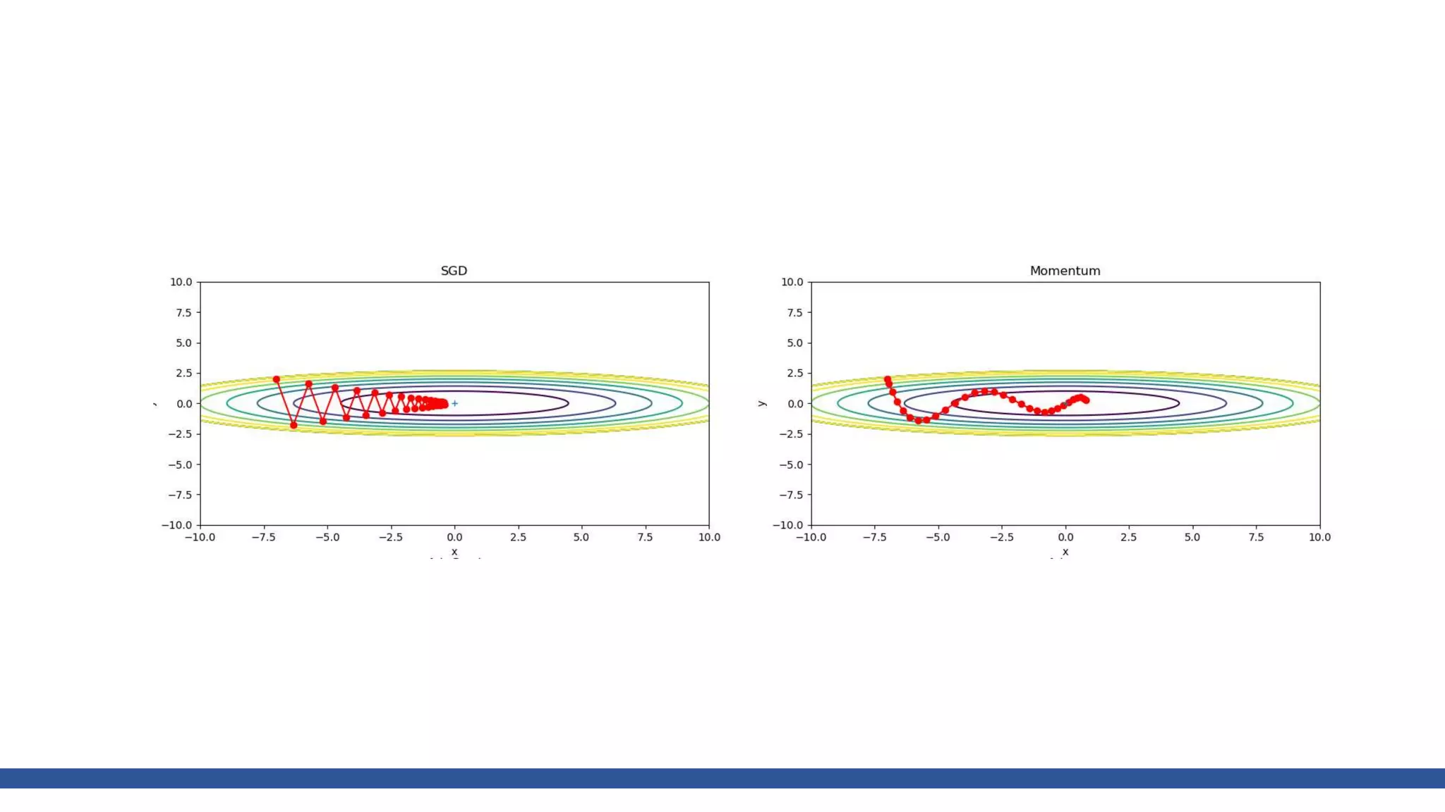
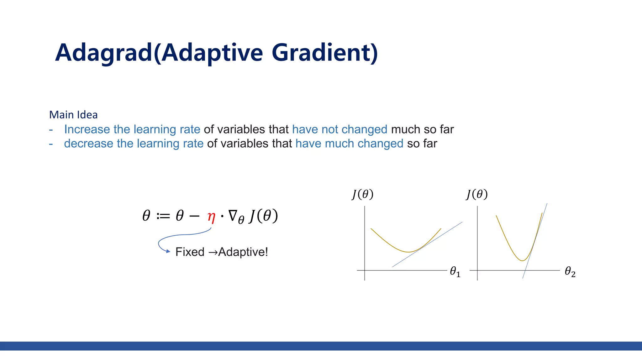
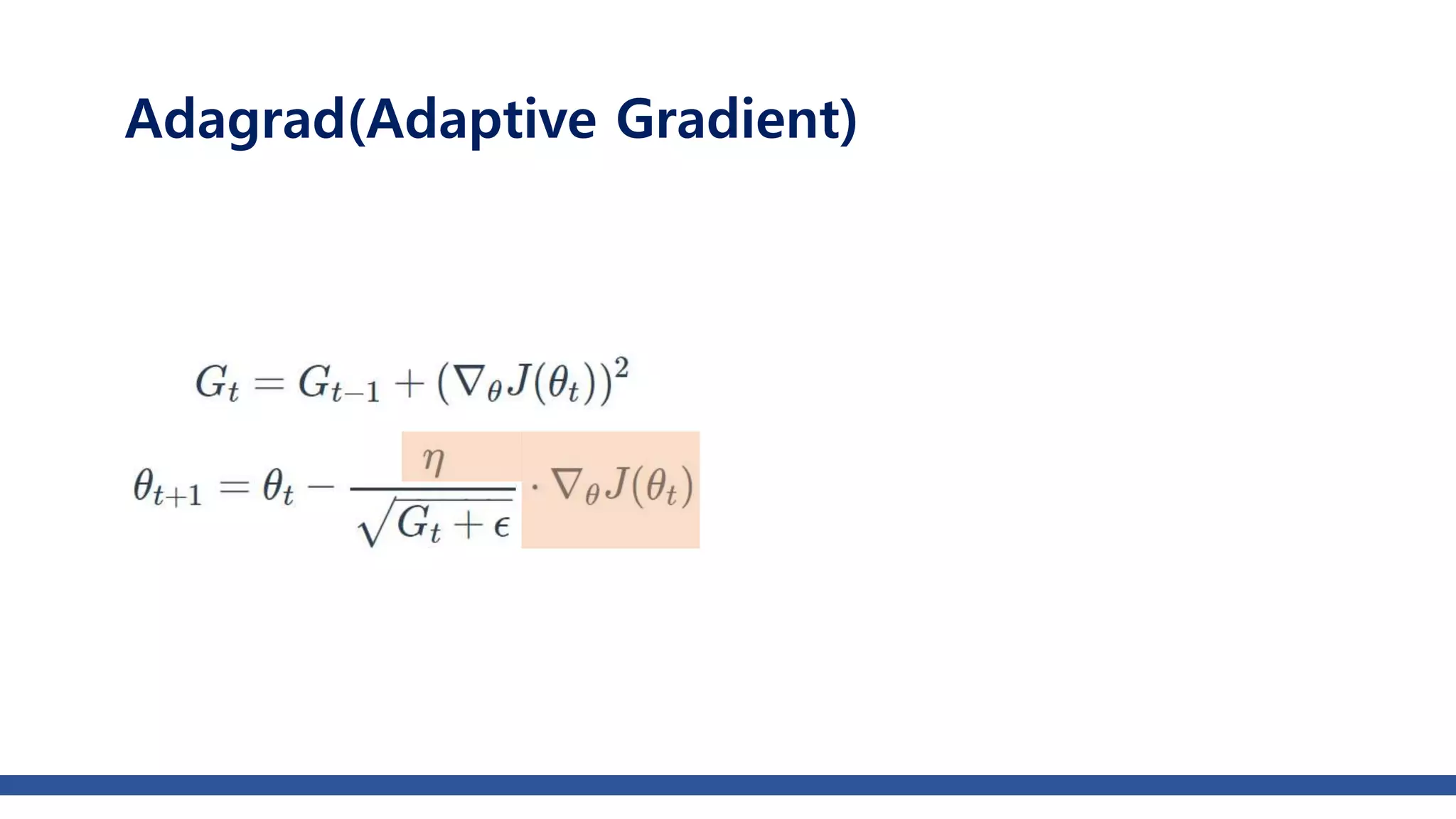
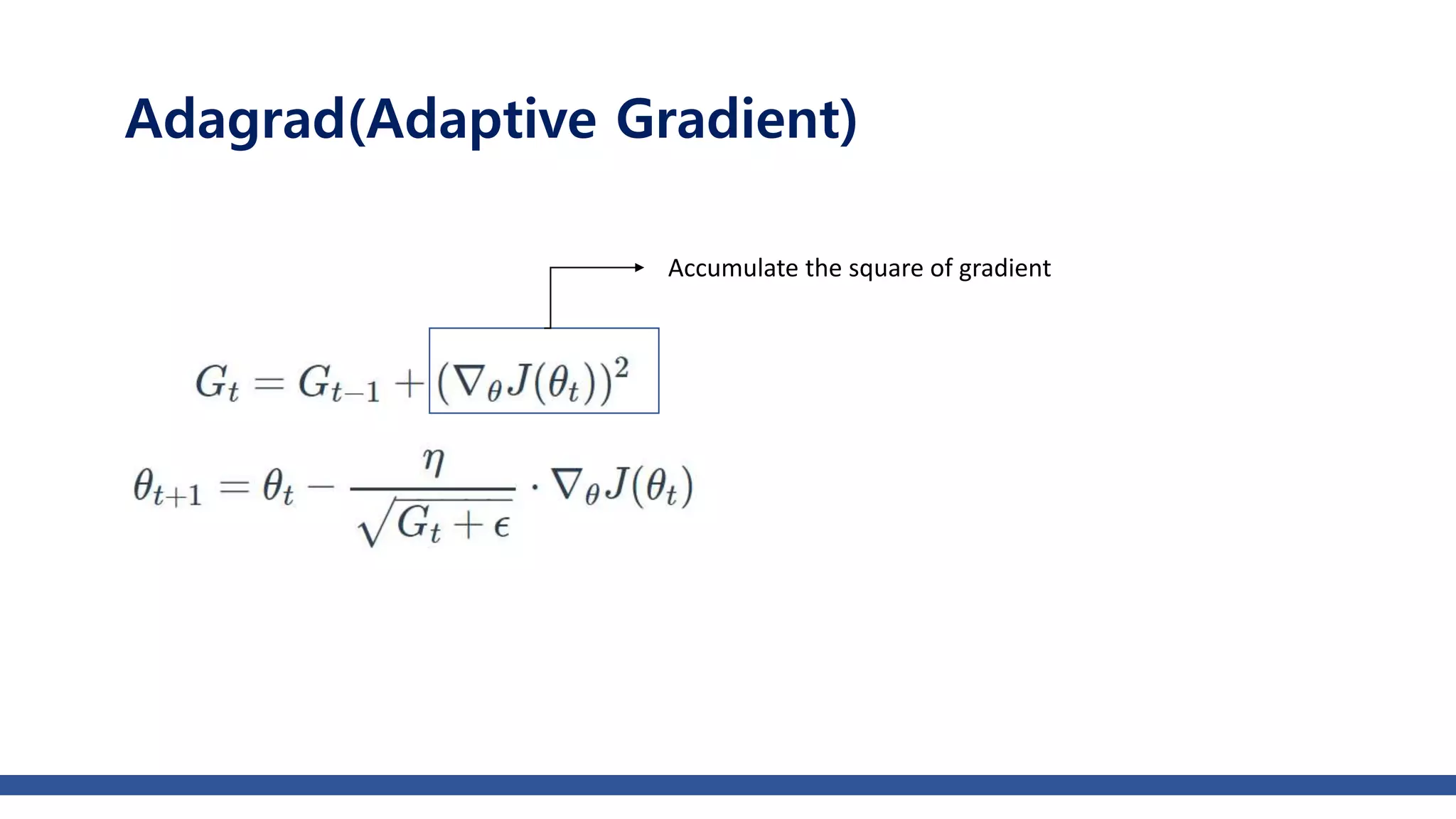
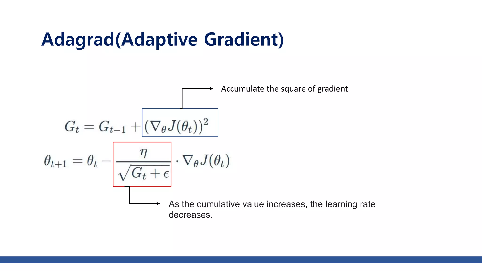
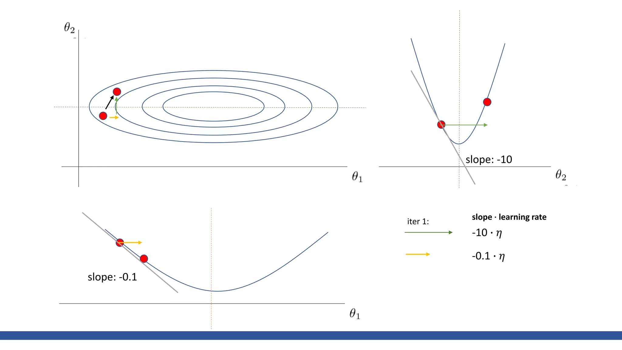
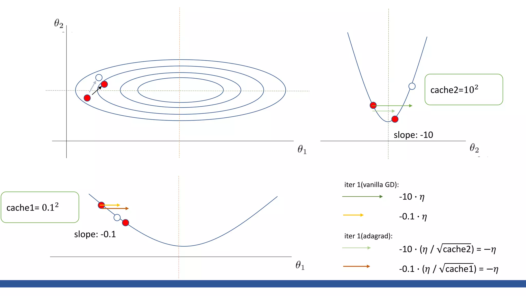
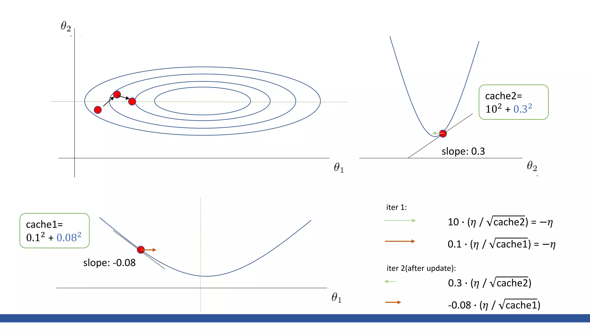
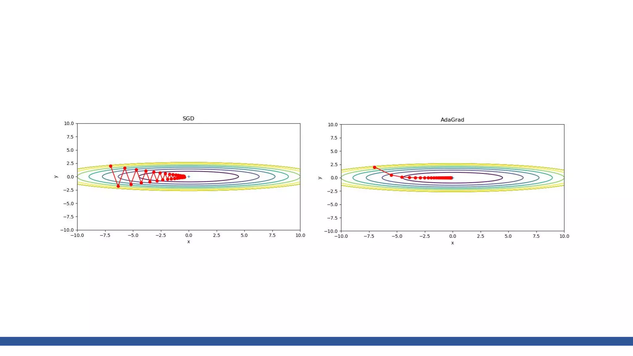
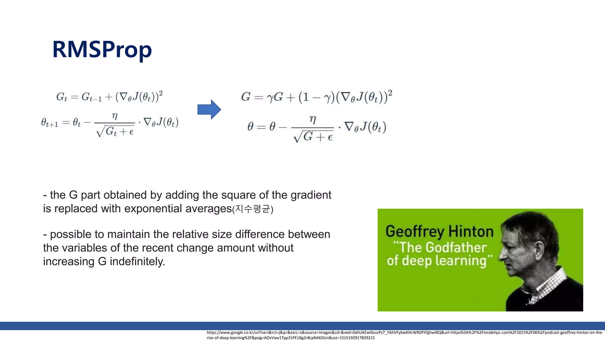
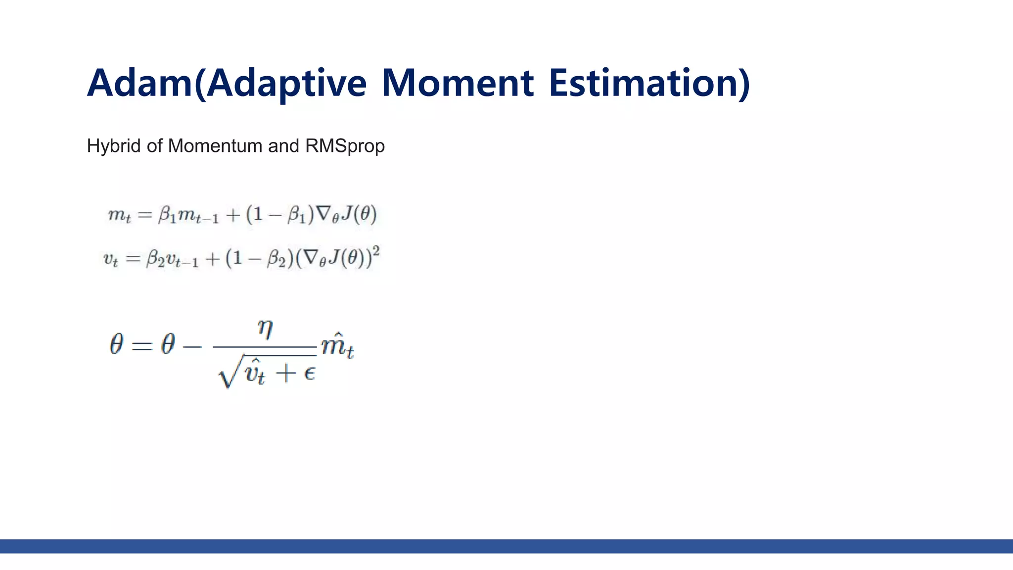
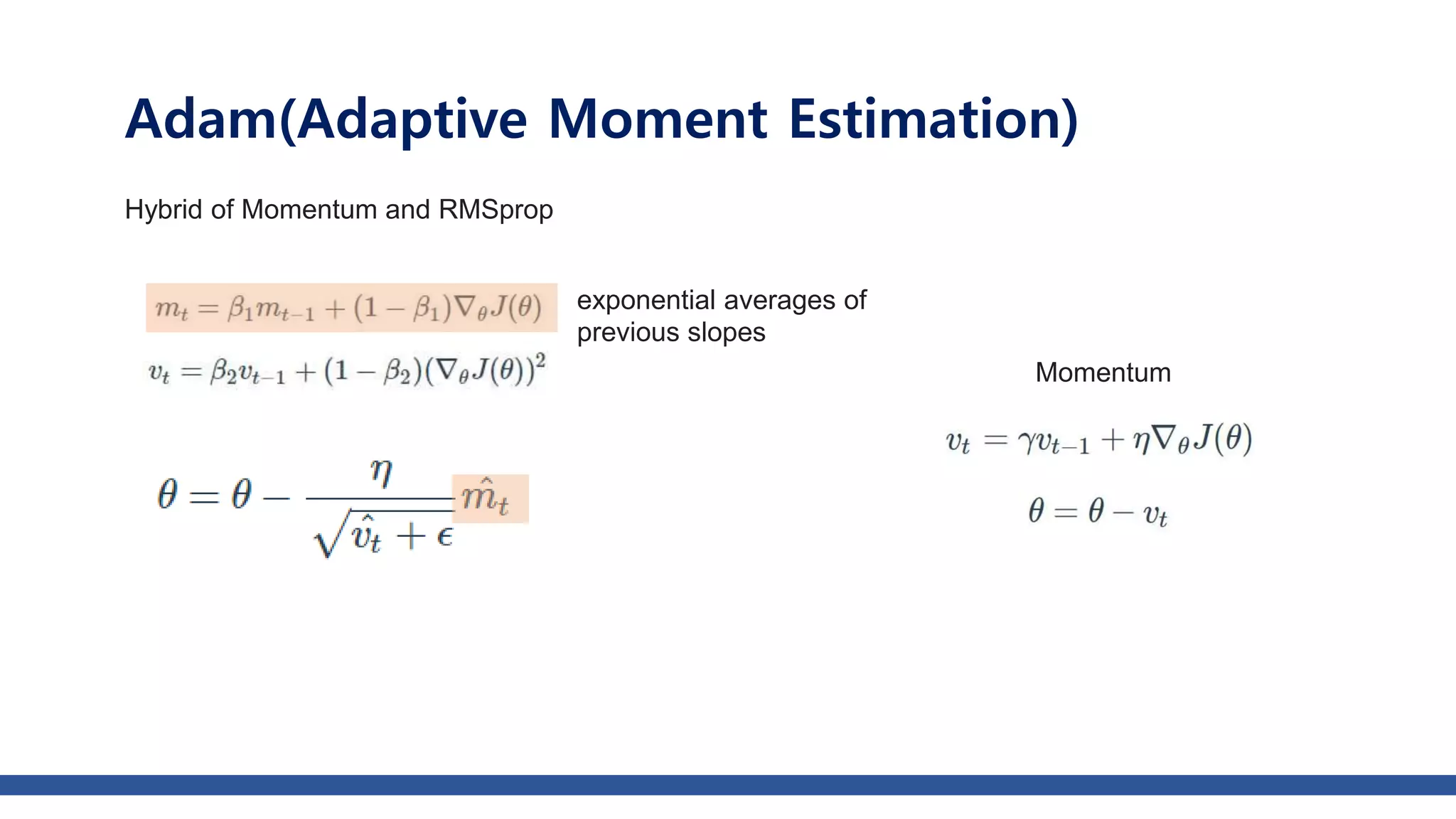
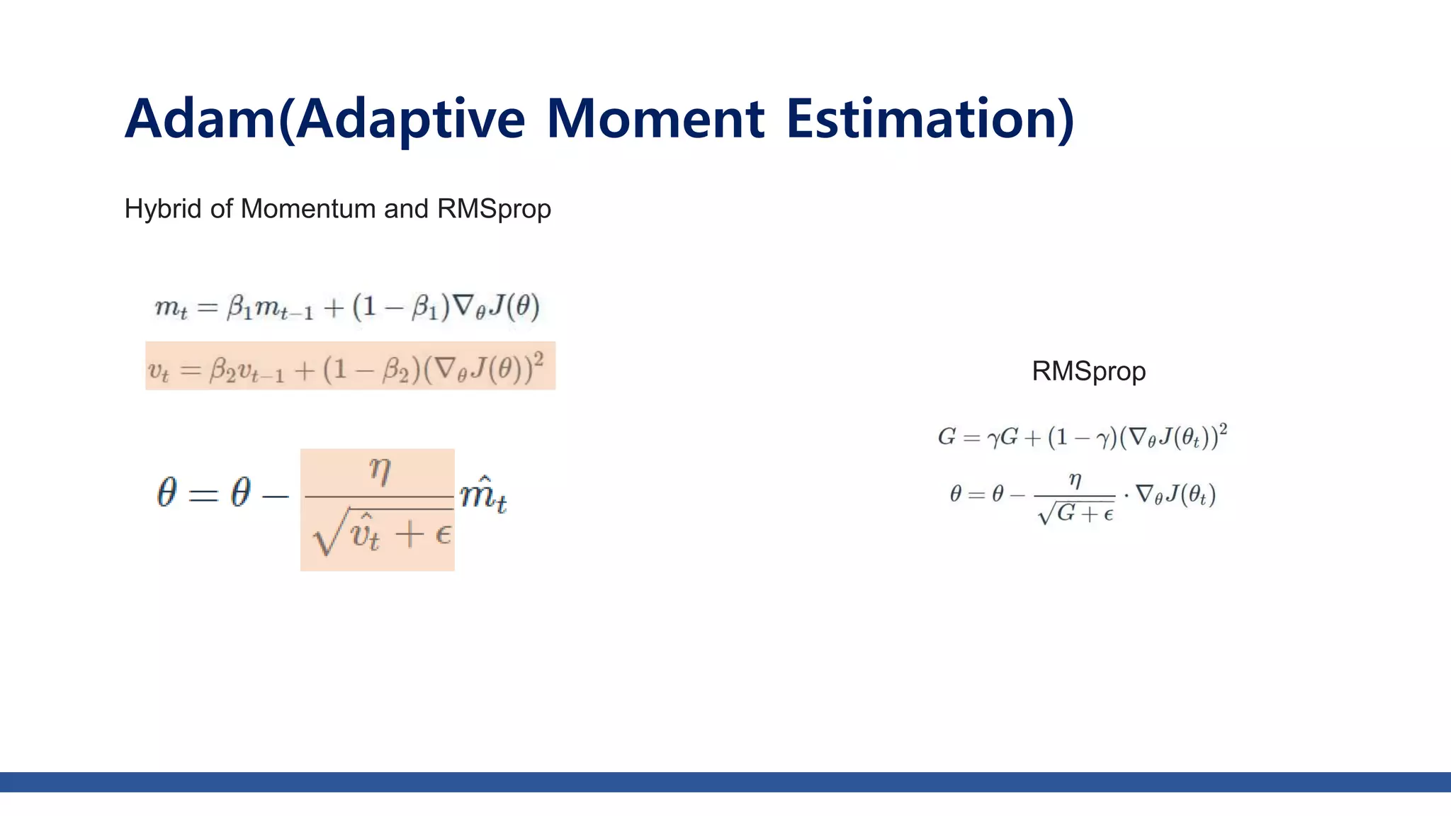
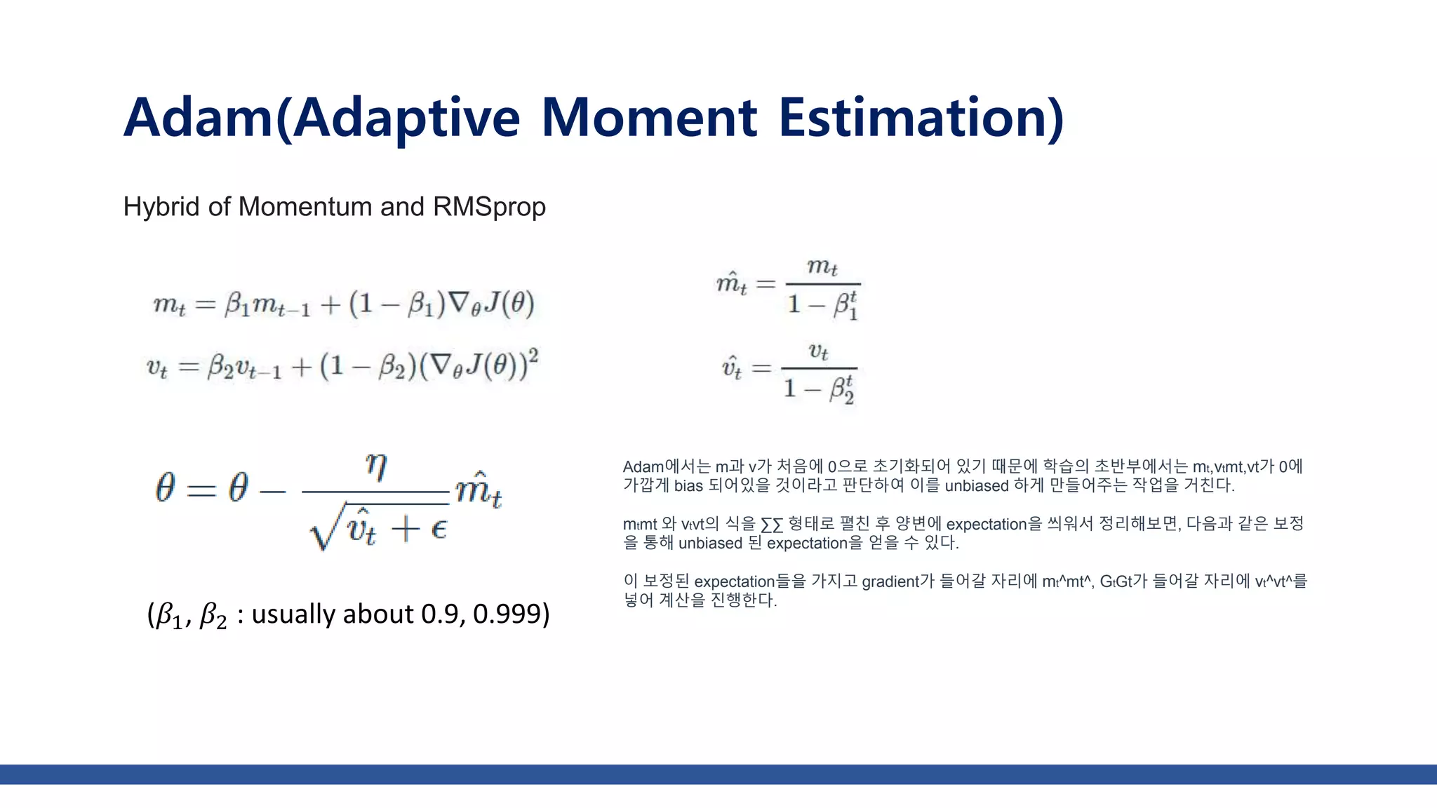
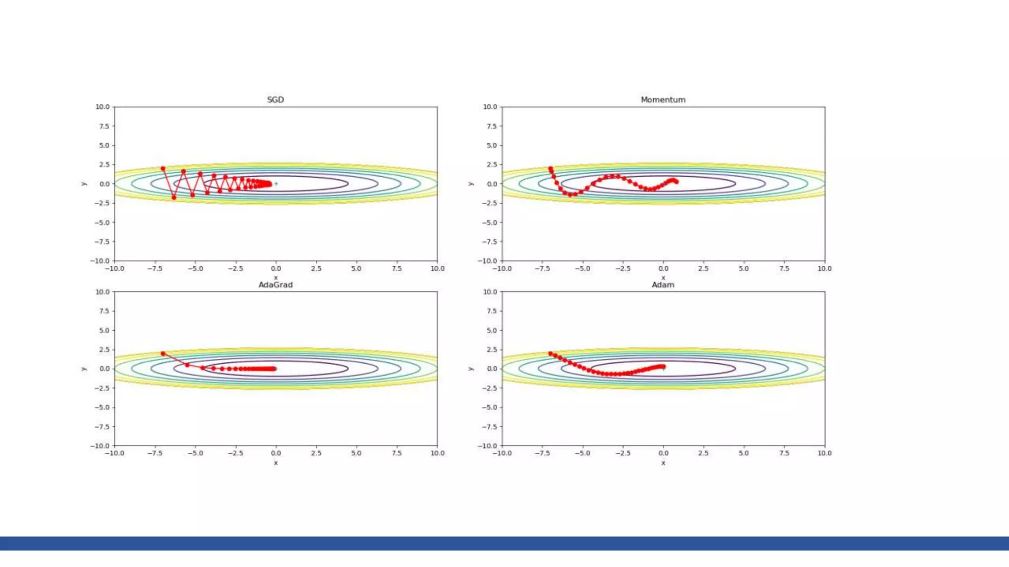
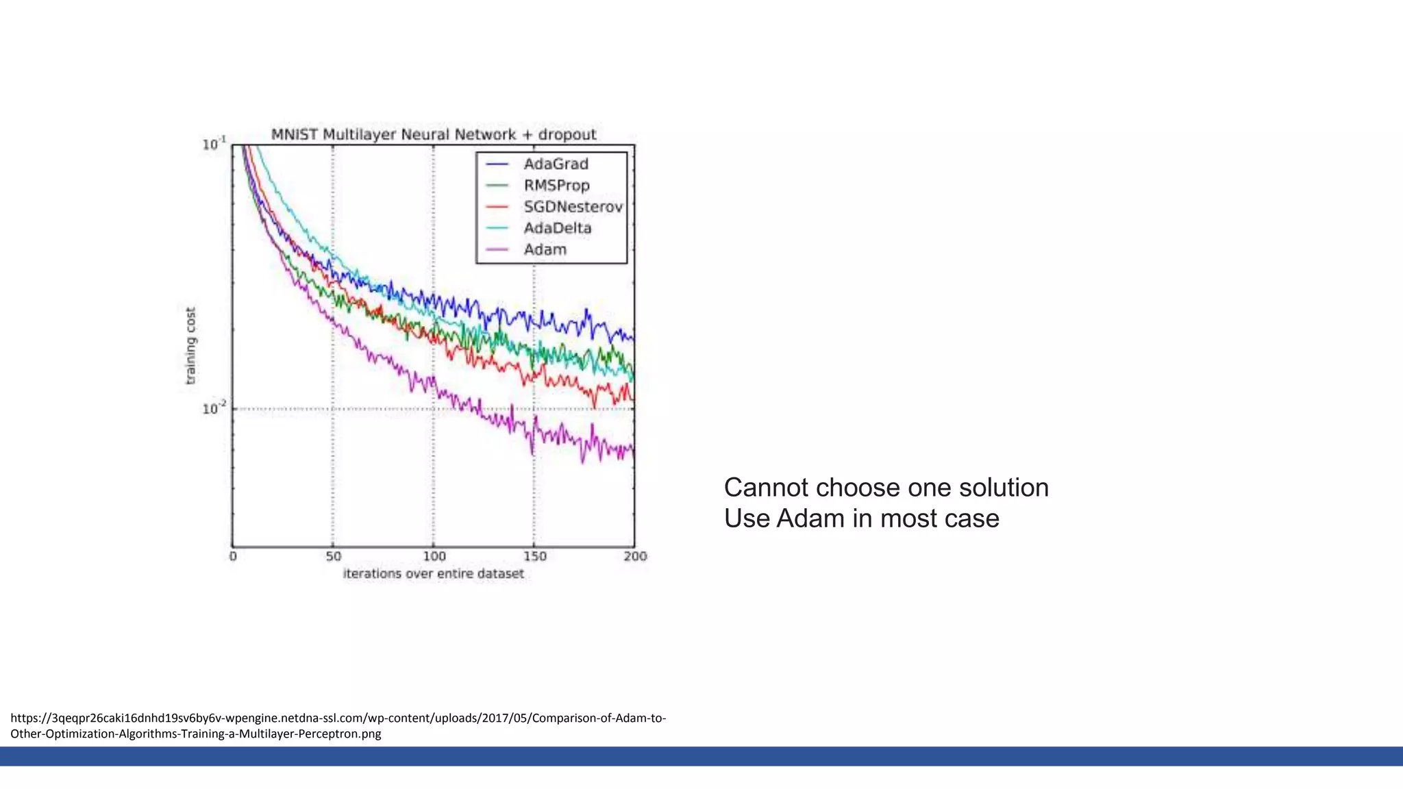
The document discusses various gradient descent optimization techniques used in machine learning, specifically batch, mini-batch, and stochastic gradient descent methods. It elaborates on advanced optimization algorithms like momentum, Adagrad, RMSProp, and Adam, explaining their mechanisms and applications. Each method aims to improve the convergence while minimizing a given loss function, with considerations for learning rate and gradients.

![class SGD:
def __init__(self, lr=0.01):
self.lr = lr
def update(self, params, grads):
for key in params.keys():
params[key] -= self.lr * grads[key]
Python
class
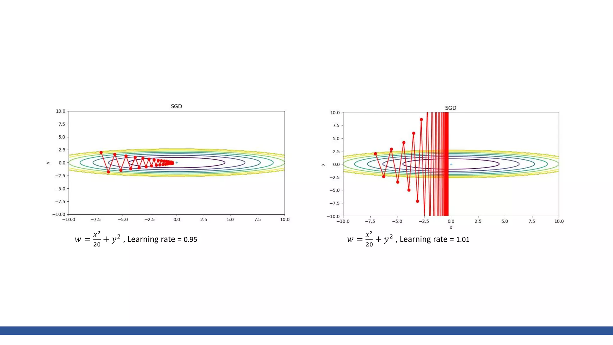
𝑤 =
𝑥2
20
+ 𝑦2
, Learning rate = 0.95, iter=30
https://github.com/WegraLee](https://image.slidesharecdn.com/gradientdescentoptimizer-180202151844/75/Gradient-descent-optimizer-16-2048.jpg)
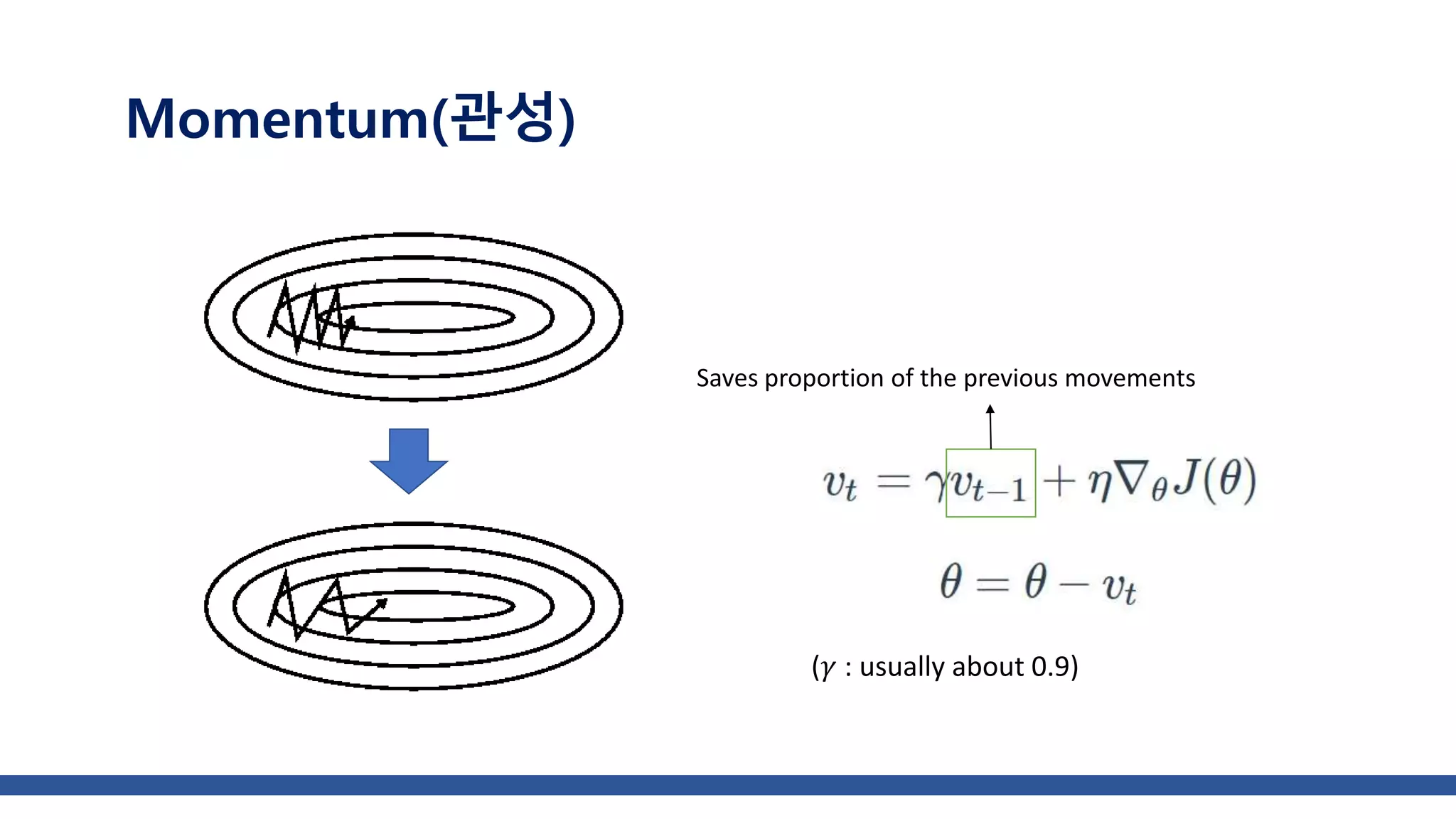
![class Momentum:
def __init__(self, lr=0.01, momentum=0.9):
self.lr = lr
self.momentum = momentum
self.v = None
def update(self, params, grads):
if self.v is None:
self.v = {}
for key, val in params.items():
self.v[key] = np.zeros_like(val)
for key in params.keys():
self.v[key] = self.momentum*self.v[key] - self.lr*grads[key]
params[key] += self.v[key]
Python
class
https://github.com/WegraLee](https://image.slidesharecdn.com/gradientdescentoptimizer-180202151844/75/Gradient-descent-optimizer-35-2048.jpg)
![W_decode = tf.Variable(tf.random_normal([n_hidden,n_input]))
b_decode = tf.Variable(tf.random_normal([n_input]))
decoder = tf.nn.sigmoid(tf.matmul(encoder,W_decode)+b_decode)
cost = tf.reduce_mean(tf.pow(X-decoder,2))
optimizer = tf.train.MomentumOptimizer(learning_rate, momentum).minimize(cost)
init = tf.global_variables_initializer()
sess = tf.Session()
sess.run(init)
Tensor flow](https://image.slidesharecdn.com/gradientdescentoptimizer-180202151844/75/Gradient-descent-optimizer-36-2048.jpg)
![class AdaGrad:
def __init__(self, lr=0.01):
self.lr = lr
self.h = None
def update(self, params, grads):
if self.h is None:
self.h = {}
for key, val in params.items():
self.h[key] = np.zeros_like(val)
for key in params.keys():
self.h[key] += grads[key] * grads[key]
params[key] -= self.lr * grads[key] / (np.sqrt(self.h[key]) + 1e-7)
Python
class
https://github.com/WegraLee](https://image.slidesharecdn.com/gradientdescentoptimizer-180202151844/75/Gradient-descent-optimizer-45-2048.jpg)
![W_decode = tf.Variable(tf.random_normal([n_hidden,n_input]))
b_decode = tf.Variable(tf.random_normal([n_input]))
decoder = tf.nn.sigmoid(tf.matmul(encoder,W_decode)+b_decode)
cost = tf.reduce_mean(tf.pow(X-decoder,2))
optimizer = tf.train.AdagradOptimizer(learning_rate,initial_accumulator_value).minimize(cost)
init = tf.global_variables_initializer()
sess = tf.Session()
sess.run(init)
Tensor flow](https://image.slidesharecdn.com/gradientdescentoptimizer-180202151844/75/Gradient-descent-optimizer-46-2048.jpg)
![W_decode = tf.Variable(tf.random_normal([n_hidden,n_input]))
b_decode = tf.Variable(tf.random_normal([n_input]))
decoder = tf.nn.sigmoid(tf.matmul(encoder,W_decode)+b_decode)
cost = tf.reduce_mean(tf.pow(X-decoder,2))
optimizer = tf.train.AdamOptimizer(learning_rate, beta1, beta2, epsilon).minimize(cost)
init = tf.global_variables_initializer()
sess = tf.Session()
sess.run(init)
Tensor flow](https://image.slidesharecdn.com/gradientdescentoptimizer-180202151844/75/Gradient-descent-optimizer-53-2048.jpg)


![[DSC Europe 25] Danica Soc - The Science Behind Marketing: Experimentation me...](https://cdn.slidesharecdn.com/ss_thumbnails/c0nofsggs9gw5ucmallr-3-251216103155-56bd64d1-thumbnail.jpg?width=640&height=640&fit=bounds)

![[DSC Europe 25] Behzad Hosseini - AI Agents in the Wild: Deploying Models tha...](https://cdn.slidesharecdn.com/ss_thumbnails/3qtejajvsjqrzwfept2c-10-251212103250-7f2b1068-thumbnail.jpg?width=640&height=640&fit=bounds)
![[DSC Europe 25] Uros Pesic - The Reality of AI in Marketing.pdf](https://cdn.slidesharecdn.com/ss_thumbnails/rtkodnmtycovsllvzsyn-9-251215095918-b0c6bfe3-thumbnail.jpg?width=640&height=640&fit=bounds)


![[DSC Europe 25] Miodrag Pesovic & Vladislav Radonjic - Federated Data Archite...](https://cdn.slidesharecdn.com/ss_thumbnails/gsbe3y5it5uhndi4e08e-1-251212103249-f1008e0c-thumbnail.jpg?width=640&height=640&fit=bounds)

![[DSC Europe 25] Dunja Adzic Jovanovic - AI and Cybersecurity: Defending Data ...](https://cdn.slidesharecdn.com/ss_thumbnails/o1zylpbhrtwnixxq2xj8-7-251211083048-185086f6-thumbnail.jpg?width=640&height=640&fit=bounds)
![[DSC Europe 25] Jovan Bogicevic - Legacy to AI-Driven Defense: Transforming D...](https://cdn.slidesharecdn.com/ss_thumbnails/rsarluadt563hntyfc8q-3-251211083849-3e7bc4c0-thumbnail.jpg?width=640&height=640&fit=bounds)
![[DSC Europe 25] Jon Dajci - Bridging TradFi and DeFi: Building the Future of ...](https://cdn.slidesharecdn.com/ss_thumbnails/fqmhfvlbqhkihjvqvhmu-7-251211083849-6af7e325-thumbnail.jpg?width=640&height=640&fit=bounds)
![[DSC Europe 25] Branko Urosevic -Rethinking Financial Talent: Integrating Cod...](https://cdn.slidesharecdn.com/ss_thumbnails/8jjrus8ttko6qj64f58f-3-251212103250-642c6374-thumbnail.jpg?width=640&height=640&fit=bounds)
![[DSC Europe 25] Dusan Nesic - Securing Tomorrow’s Infrastructure: Why Cyber-P...](https://cdn.slidesharecdn.com/ss_thumbnails/qikbszfftyowjm2q6duw-1-251211083848-8f2ead6b-thumbnail.jpg?width=640&height=640&fit=bounds)
![[DSC Europe 25] Nikolay Burlutskiy - Best Practices for Building Enterprise M...](https://cdn.slidesharecdn.com/ss_thumbnails/uirvaiuvq8y1w8hzd9tx-7-251212103249-2619edb4-thumbnail.jpg?width=640&height=640&fit=bounds)