Download to read offline
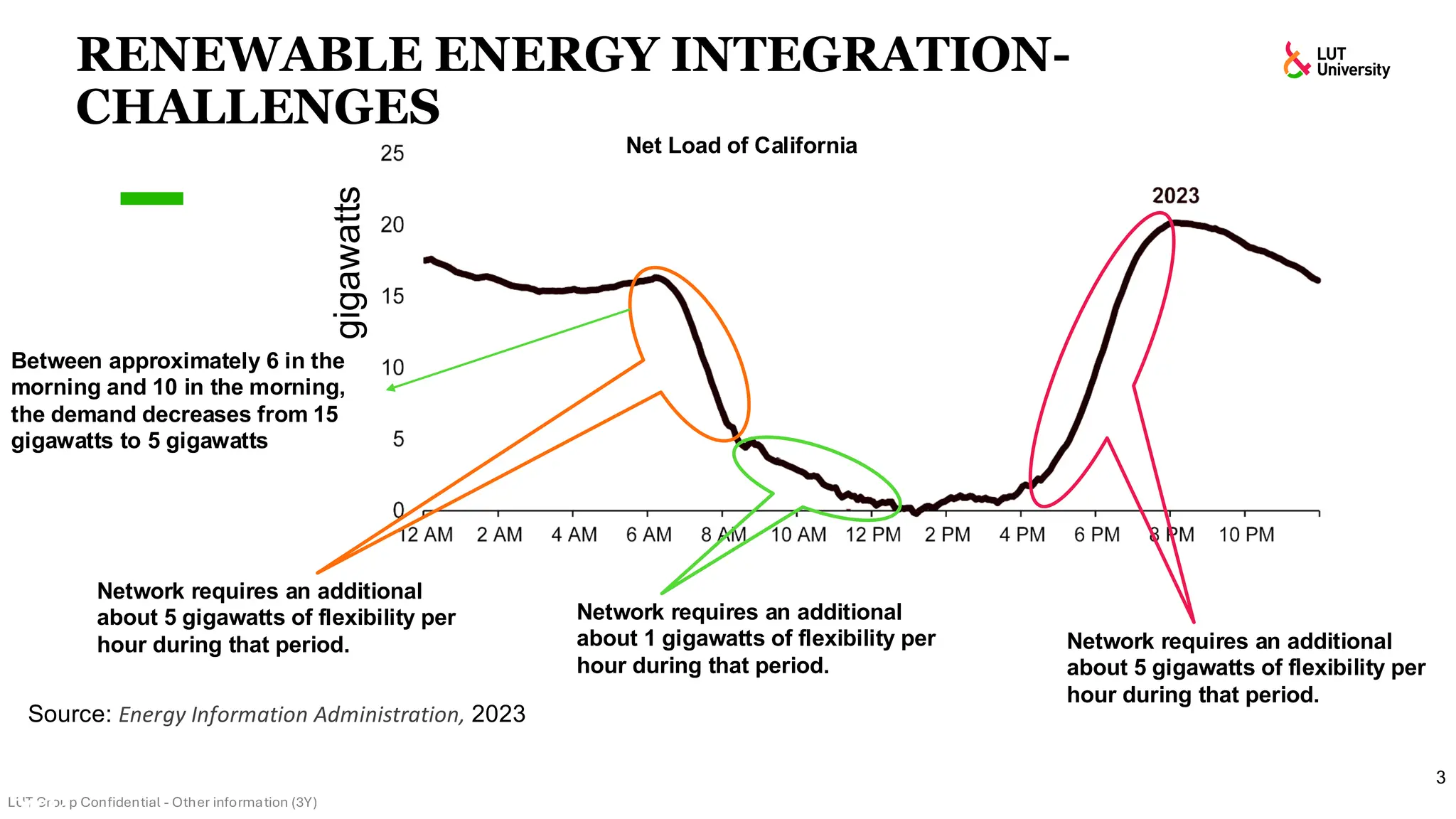
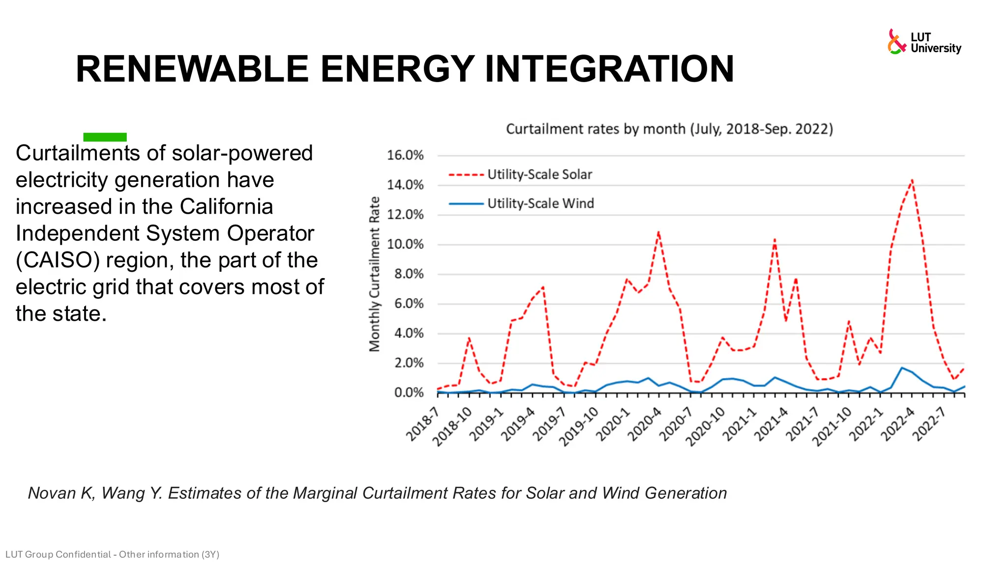
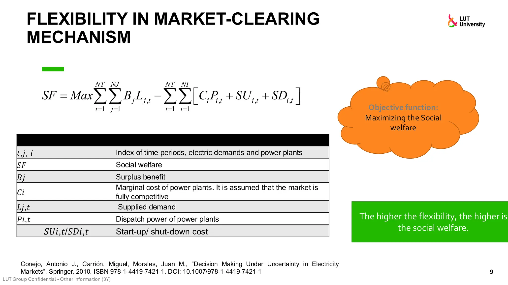
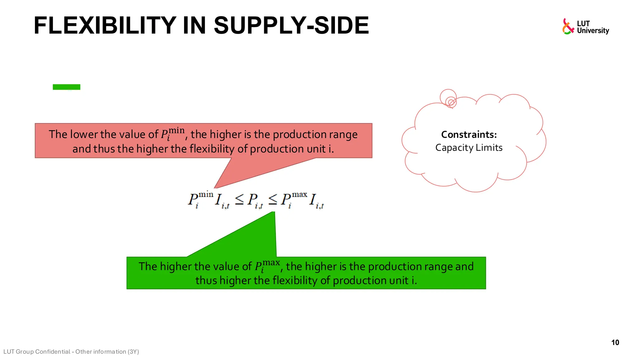
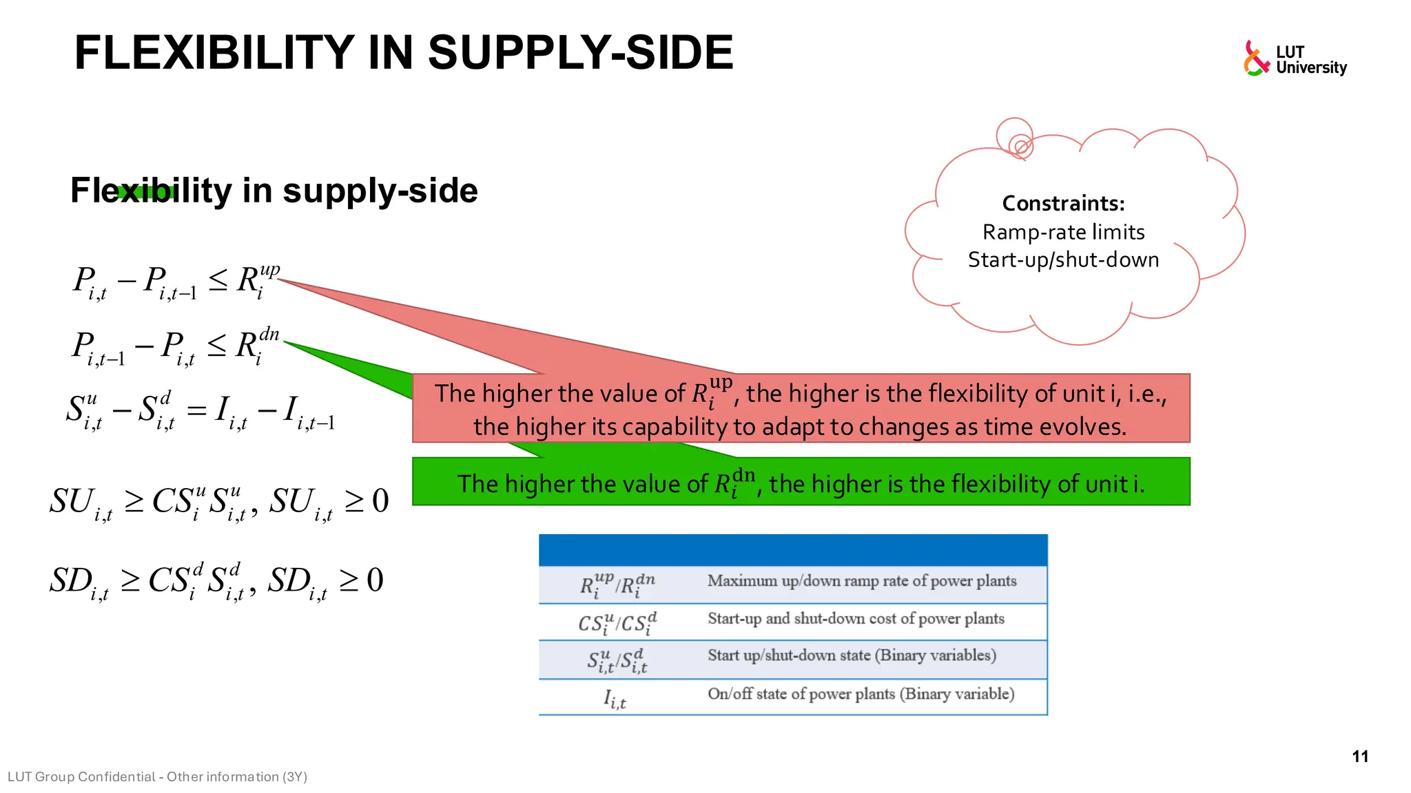
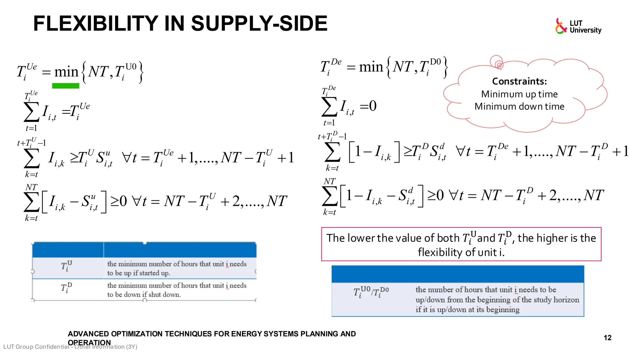
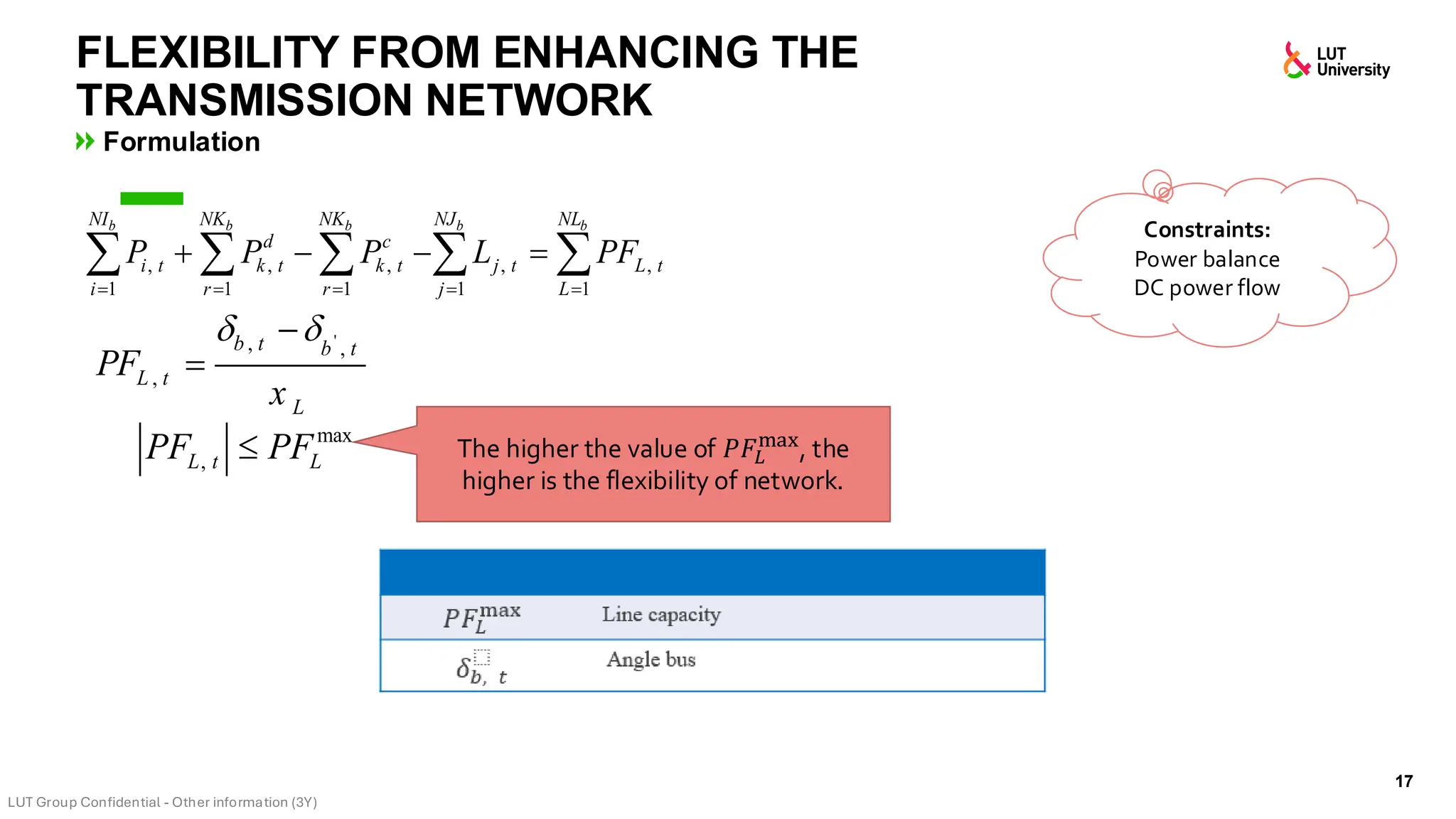
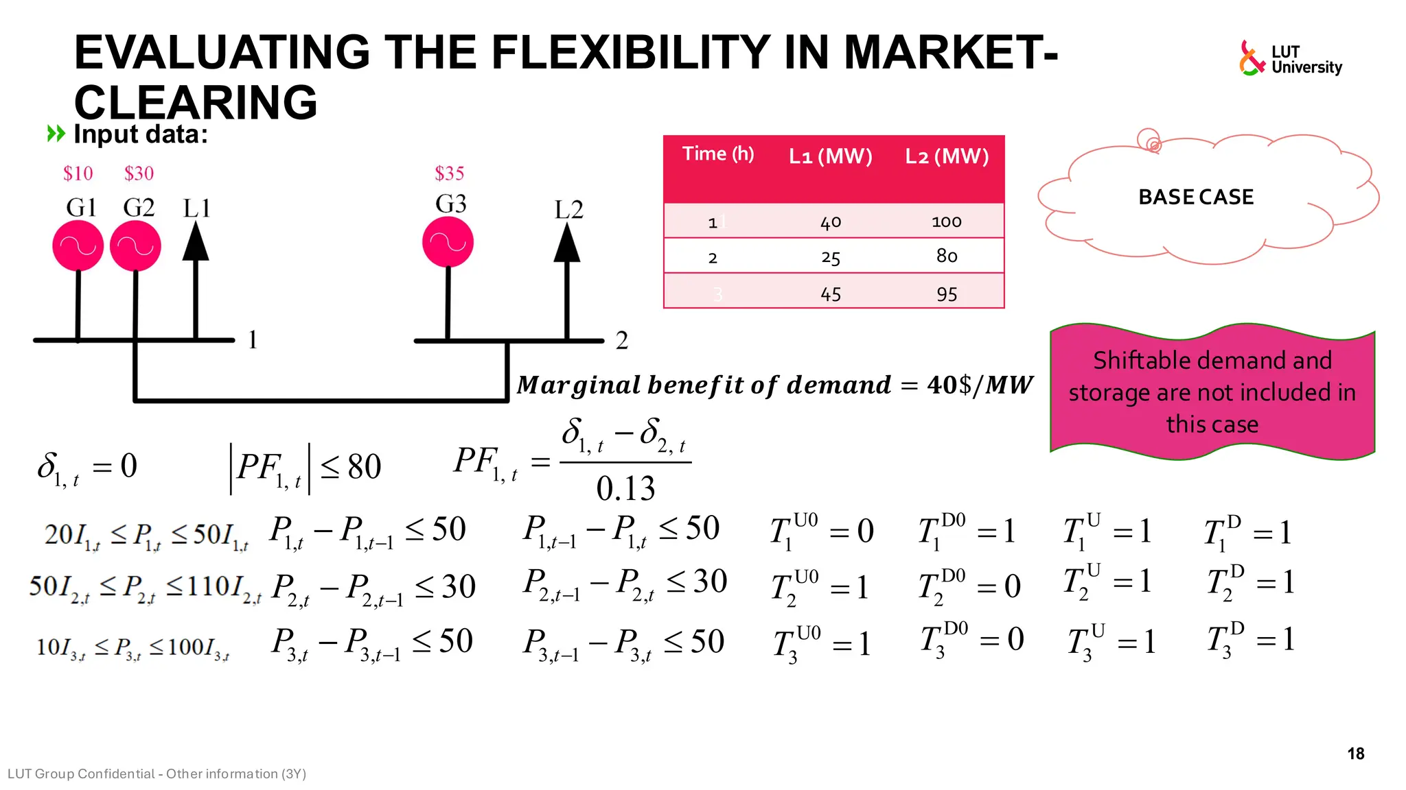
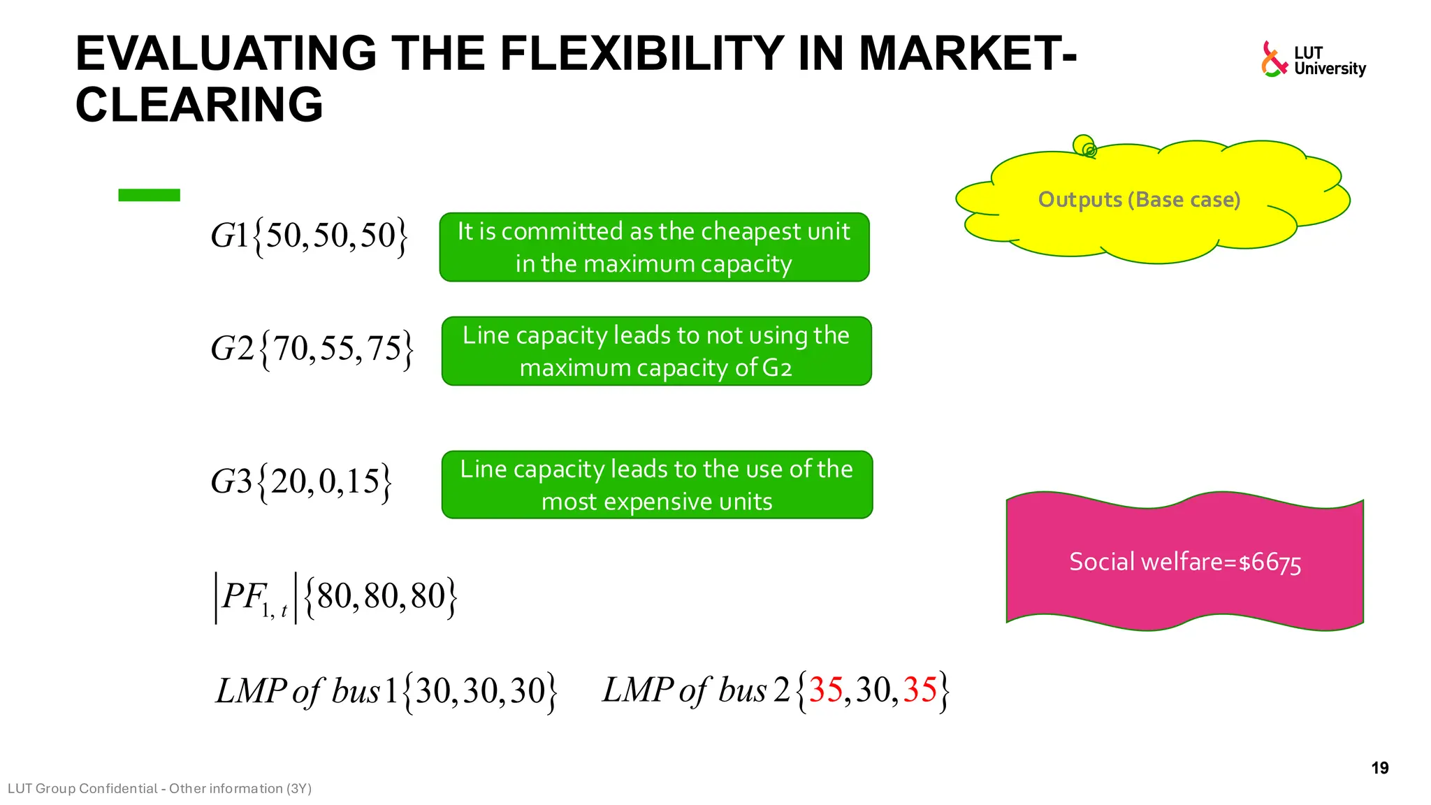
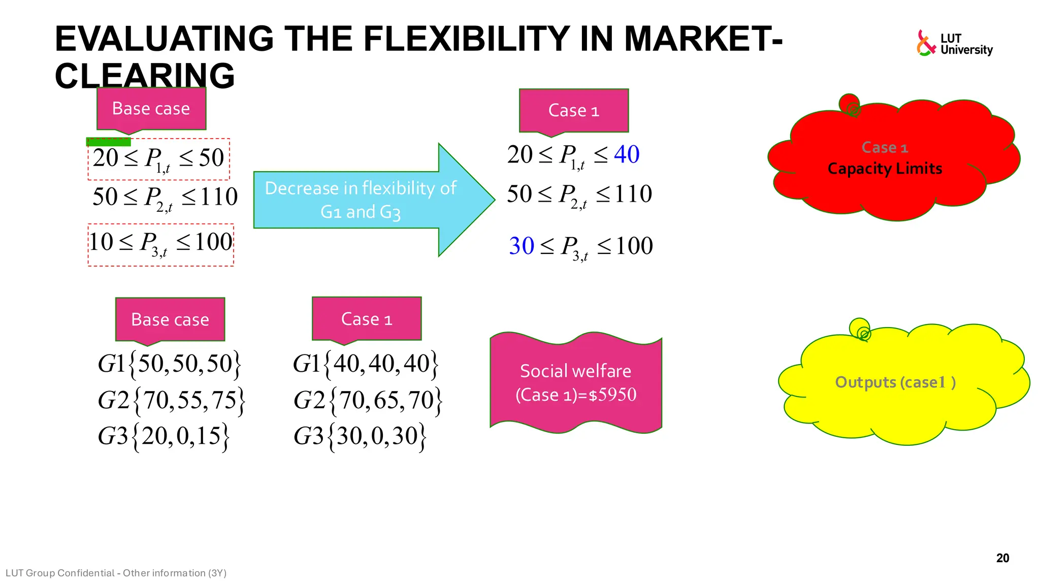
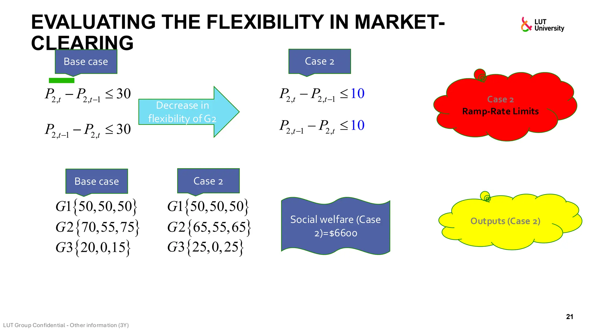
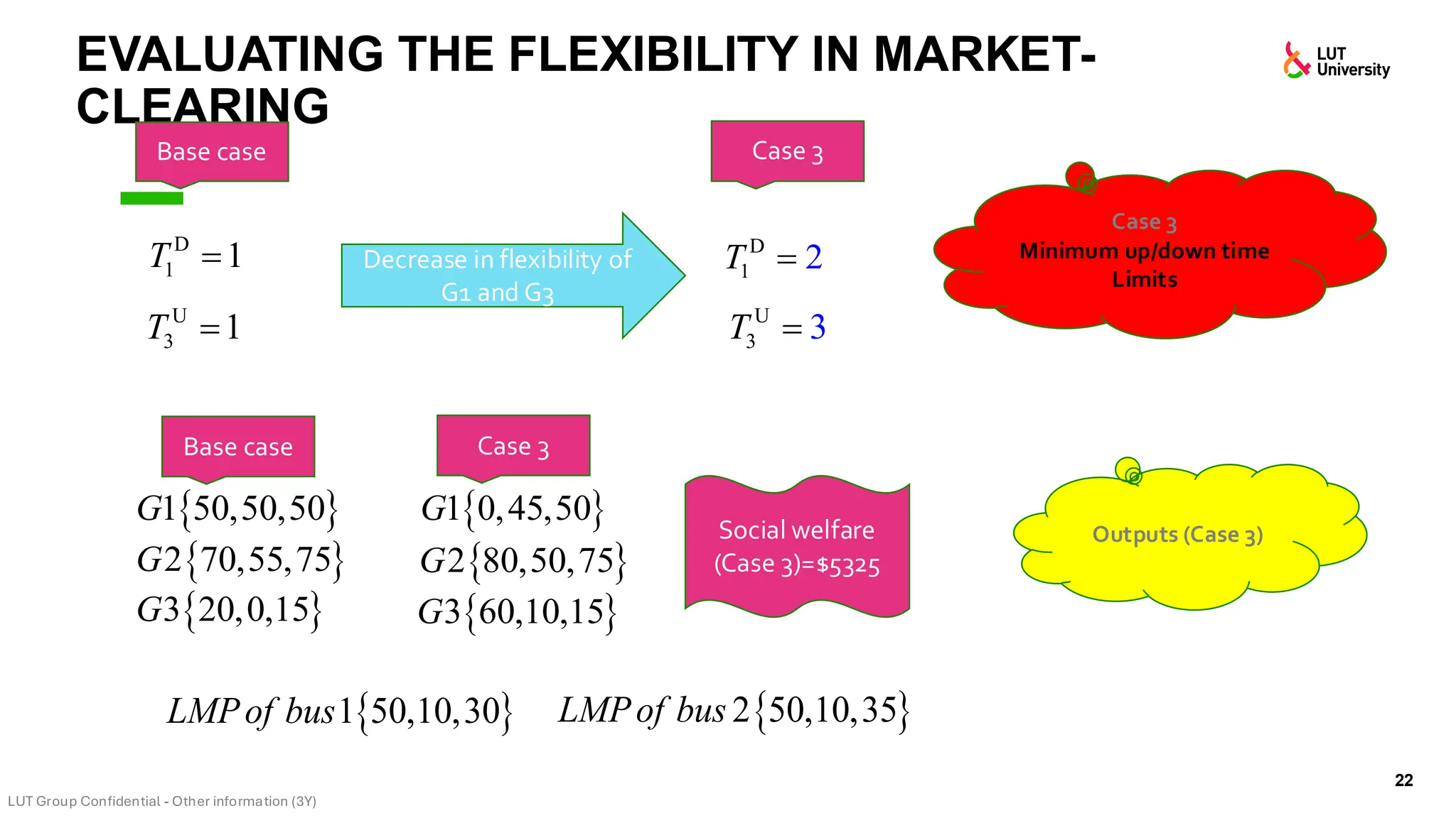
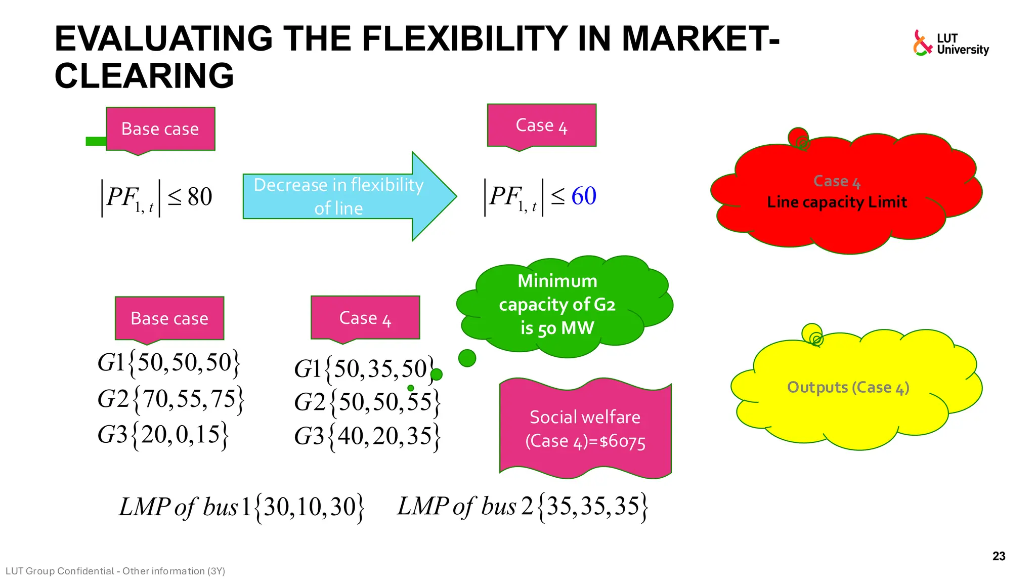
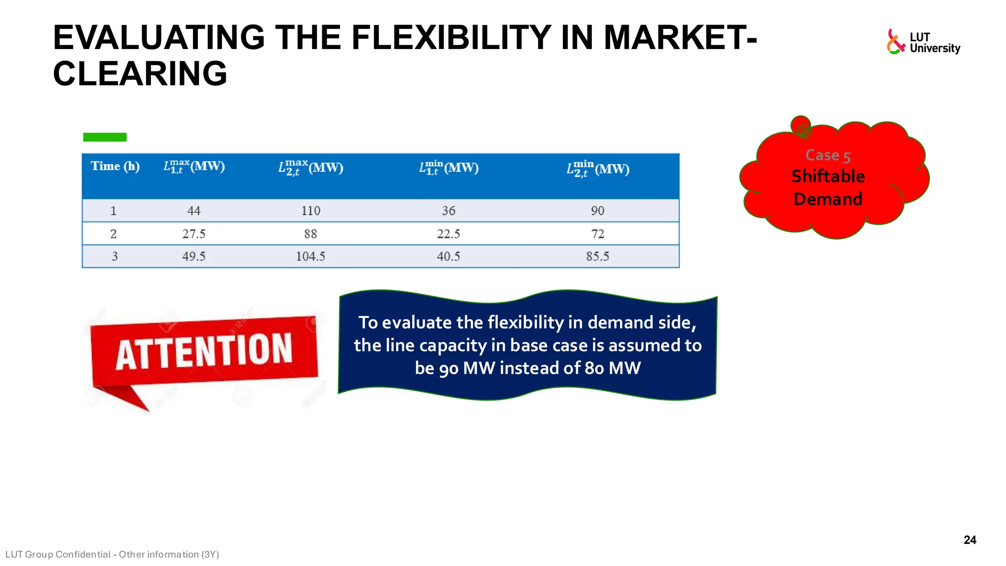
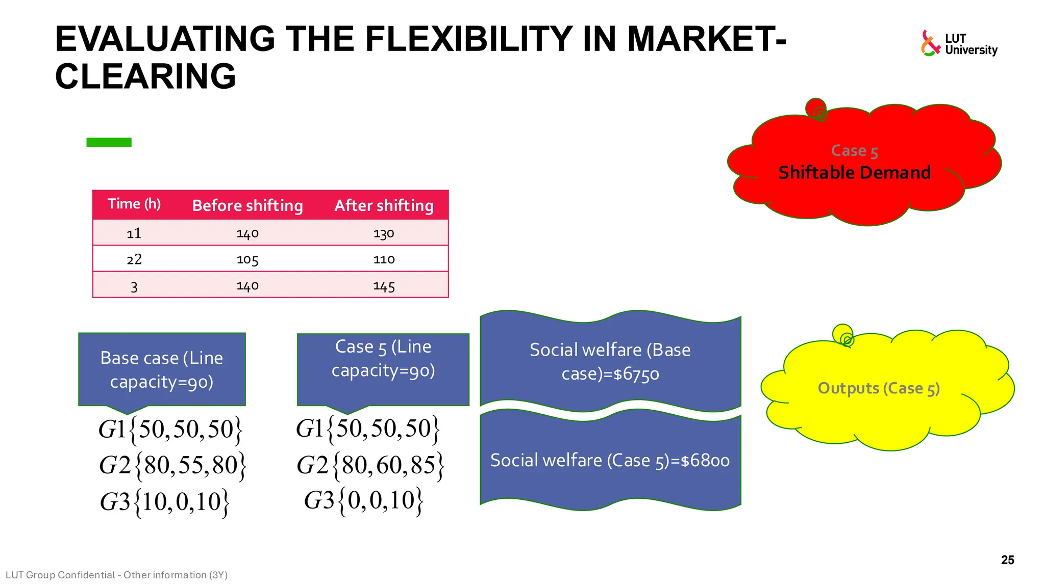
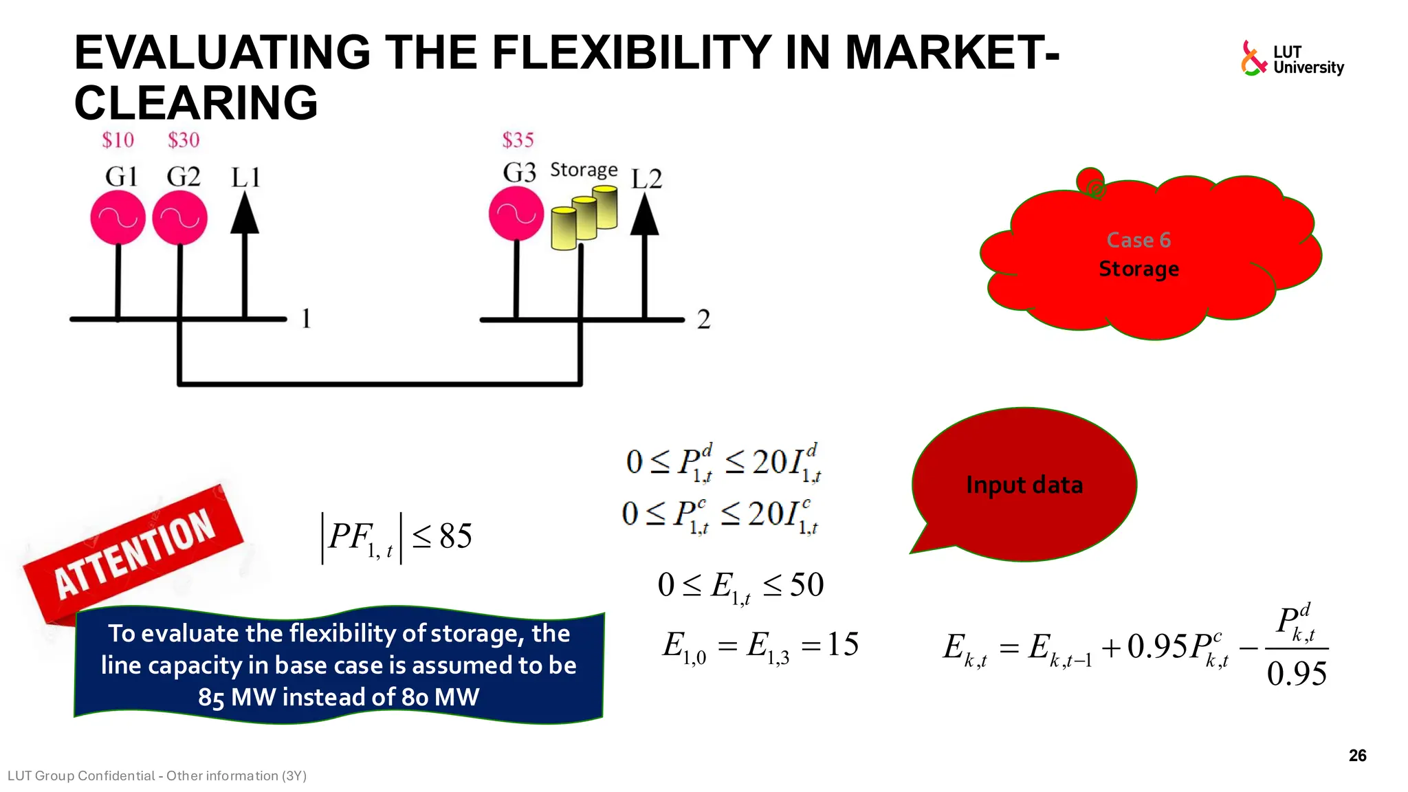
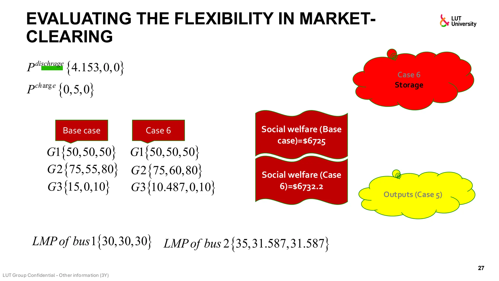


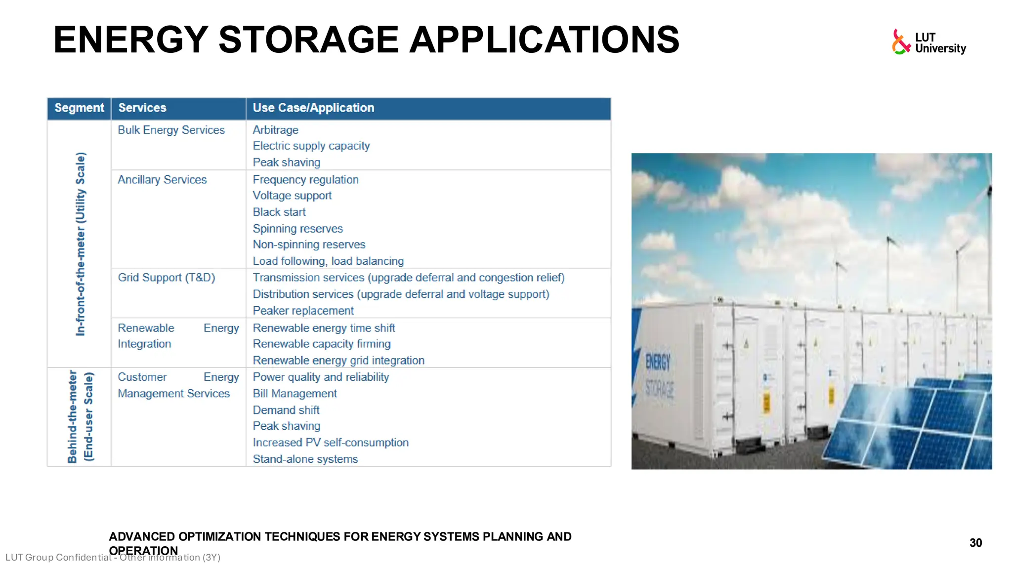


This slide-deck is a concise walkthrough of why high renewable penetration creates operational challenges (e.g., net-load “duck curve” flexibility needs and increasing curtailment), and how power systems respond through flexibility from the supply side, demand side, storage, and transmission. It introduces key operational optimization problems like (network-constrained) unit commitment, highlights the explosion of complexity with larger networks, and frames market-clearing as social welfare maximization with practical constraints (capacity, ramping, min up/down time, reserves, and power flow). The deck then uses step-by-step case studies to show how tightening/relaxing constraints (generator limits, ramps, min up/down time, line capacity) and adding shiftable demand or storage changes dispatch outcomes, prices, and welfare.


![[2020.2] PSOC - Unit_Commitment.pptx](https://cdn.slidesharecdn.com/ss_thumbnails/2020-230328034214-f9eb2e64-thumbnail.jpg?width=640&height=640&fit=bounds)


