Evolutionary Algorithms
Evolutionaryalgorithms (EAs) are a type of metaheuristic
algorithm that are inspired by the process of natural evolution.
They are used to find optimal solutions to problems that are
difficult to solve using traditional methods.
EAs work by creating a population of solutions, and then
iteratively improving those solutions over time. Each solution in
the population is represented as a chromosome, which is a string
of genes. The genes in the chromosome represent the different
parameters of the solution.
3.
EAs have beenused to solve a wide
variety of problems, including:
* Optimization problems
* Machine learning problems
* Engineering design problems
* Financial planning problems
* Natural language processing problems
* Computer vision problems
Optimization
Optimization isthe process of finding
the best solution out of all feasible
solutions.
The aim of optimization is to find an
algorithm which solves a given class of
problems.
There exists no specific method which
solves effectively all optimization
problems (No free launch theorems).
5
6.
Classification of optimization
problems
1.Depending on the nature of equations involved in the
objective function and constraints:
Linear optimization problem
Non-linear optimization problem
6
7.
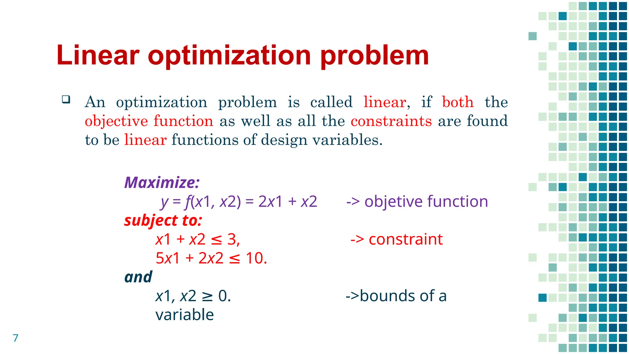
Linear optimization problem
An optimization problem is called linear, if both the
objective function as well as all the constraints are found
to be linear functions of design variables.
Maximize:
y = f(x1, x2) = 2x1 + x2 -> objetive function
subject to:
x1 + x2 ≤ 3, -> constraint
5x1 + 2x2 ≤ 10.
and
x1, x2 ≥ 0. ->bounds of a
variable
7
8.
Non-linear optimization problem
An optimization problem is called non-linear, if any one or
both of the objective function and the constraints are
found to be non-linear functions of design variables.
Maximize:
y = f(x1, x2) =+
subject to:
+ ≤ 629,
+ ≤ 133,
and
x1, x2 ≥ 0.
8
9.
Classification of optimizationproblems
(cont.)
2. Based on the existence of any functional constraint:
Un constrained optimization problem.
Constrained optimization problem.
9
10.
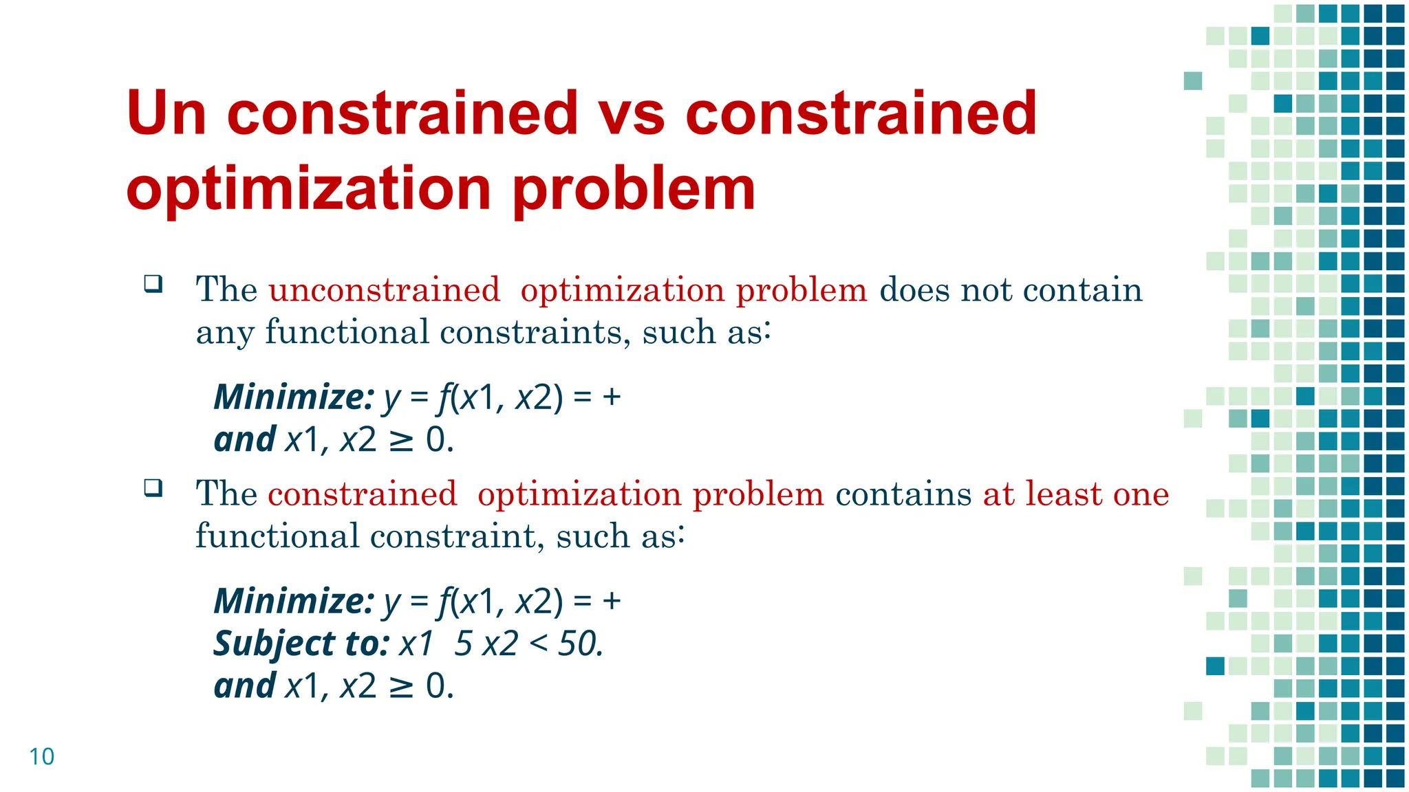
Un constrained vsconstrained
optimization problem
The unconstrained optimization problem does not contain
any functional constraints, such as:
Minimize: y = f(x1, x2) = +
and x1, x2 ≥ 0.
The constrained optimization problem contains at least one
functional constraint, such as:
Minimize: y = f(x1, x2) = +
Subject to: x1 5 x2 < 50.
and x1, x2 ≥ 0.
10
11.
Classification of optimizationproblems
(cont.)
3. Depending on the type of design variables:
Integer programming optimization problem.
Real-valued programming optimization problem.
Mixed integer programming optimization problem.
11
12.
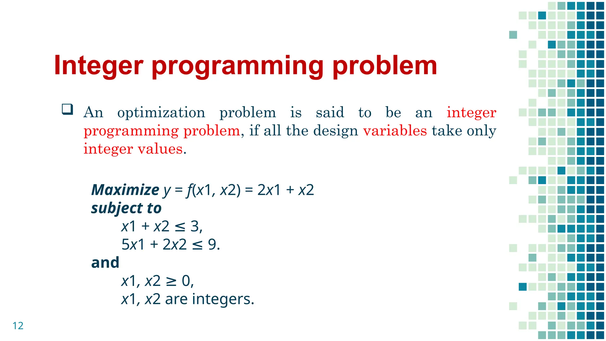
Integer programming problem
An optimization problem is said to be an integer
programming problem, if all the design variables take only
integer values.
Maximize y = f(x1, x2) = 2x1 + x2
subject to
x1 + x2 ≤ 3,
5x1 + 2x2 ≤ 9.
and
x1, x2 ≥ 0,
x1, x2 are integers.
12
13.
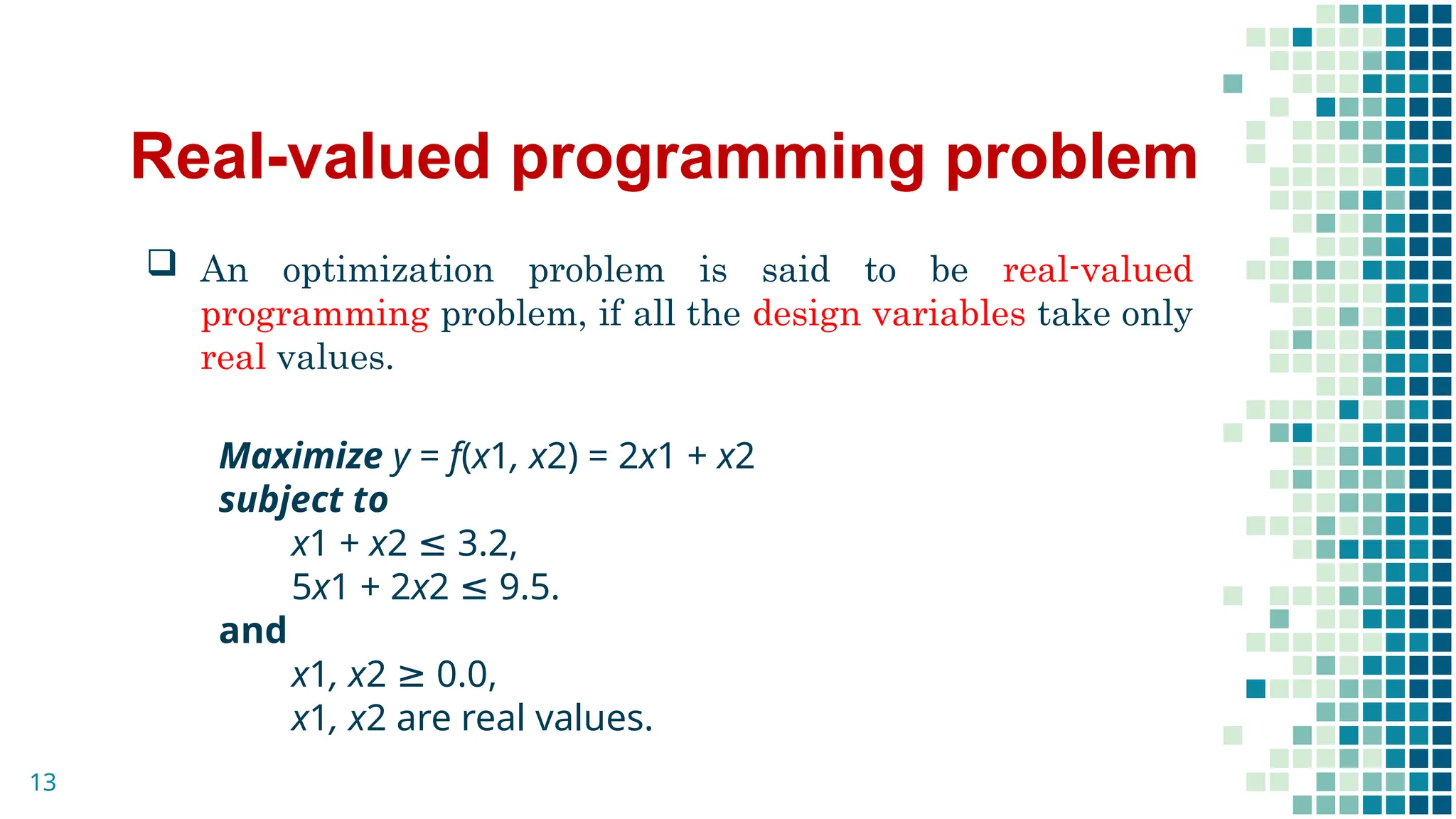
Real-valued programming problem
An optimization problem is said to be real-valued
programming problem, if all the design variables take only
real values.
Maximize y = f(x1, x2) = 2x1 + x2
subject to
x1 + x2 ≤ 3.2,
5x1 + 2x2 ≤ 9.5.
and
x1, x2 ≥ 0.0,
x1, x2 are real values.
13
14.
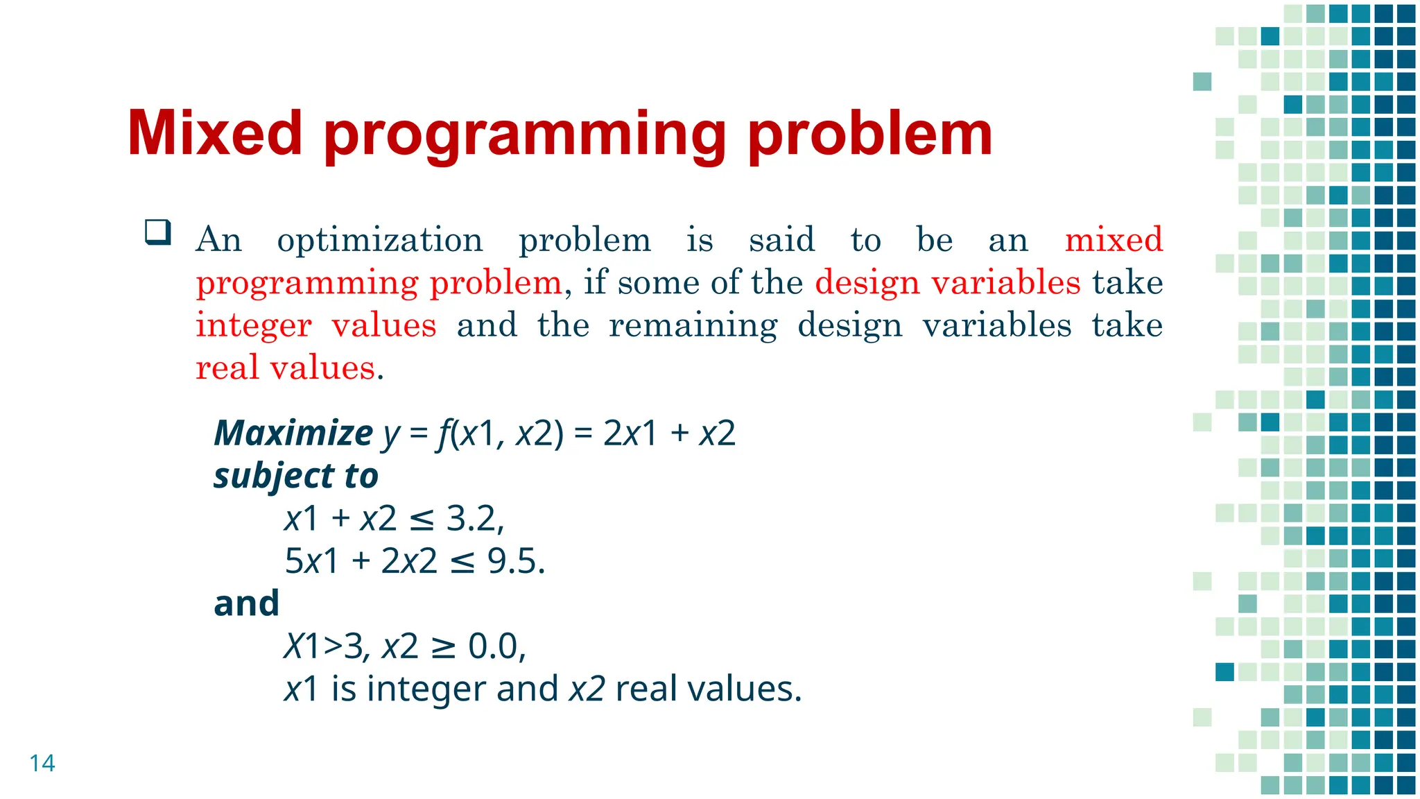
Mixed programming problem
An optimization problem is said to be an mixed
programming problem, if some of the design variables take
integer values and the remaining design variables take
real values.
Maximize y = f(x1, x2) = 2x1 + x2
subject to
x1 + x2 ≤ 3.2,
5x1 + 2x2 ≤ 9.5.
and
X1>3, x2 ≥ 0.0,
x1 is integer and x2 real values.
14
15.
Single objective vsmulti-objective
optimization problem
4. Depending on the number of objective functions:
Single optimization problem.
Multi-objective optimization problem.
Single optimization problem is a problem that contains only
one objective function to be optimized (maximized or
minimized).
Multi-objective optimization problem is a problem that has
a set or vector of conflicting objective functions to be
optimized.
15
16.
Combinatorial vs continuous
optimizationproblem
▪ Combinatorial or discrete optimization problem is an
optimization problem in which its design variables takes
discrete values.
▪ Continuous optimization problem is an optimization
problem in which its design variables takes continuous
values.
16
17.
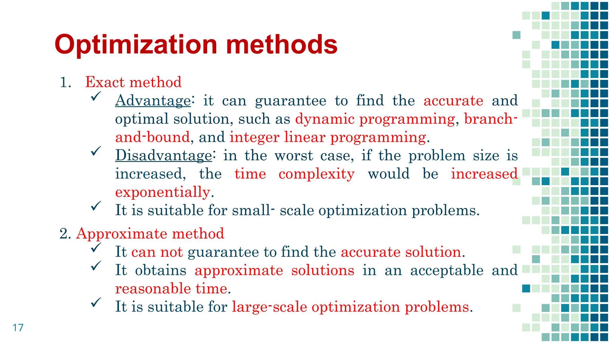
Optimization methods
1. Exactmethod
Advantage: it can guarantee to find the accurate and
optimal solution, such as dynamic programming, branch-
and-bound, and integer linear programming.
Disadvantage: in the worst case, if the problem size is
increased, the time complexity would be increased
exponentially.
It is suitable for small- scale optimization problems.
2. Approximate method
It can not guarantee to find the accurate solution.
It obtains approximate solutions in an acceptable and
reasonable time.
It is suitable for large-scale optimization problems.
17
18.
Heuristic method
Itis an approximate method designed to solve quickly the
problem, while scarifying the exact solution.
They are often problem-dependent, that is, you define a
heuristic for a given problem.
The quality of solution depends on the initial starting
points.
18
19.
Metaheuristic algorithm
Metaheuristicsare approximate methods that can not
guarantee the exact and optimal solutions.
They are problem-independent techniques that can be
applied to a broad range of problems.
For example, genetic algorithm and particle swarm
algorithms are metaheuristic algorithms.
19
Evolutionary computation
Evolutionarycomputation is a soft
computing direction that starts by
transferring the ideas of biological
evolutionary theory into computer science
to solve problems.
Charles Darwin has formulated the
fundamental principle of natural
selection as the main evolutionary tool.
Combination of Darwin’s and Mendel’s
ideas lead to the modern evolutionary
theory.
21
22.
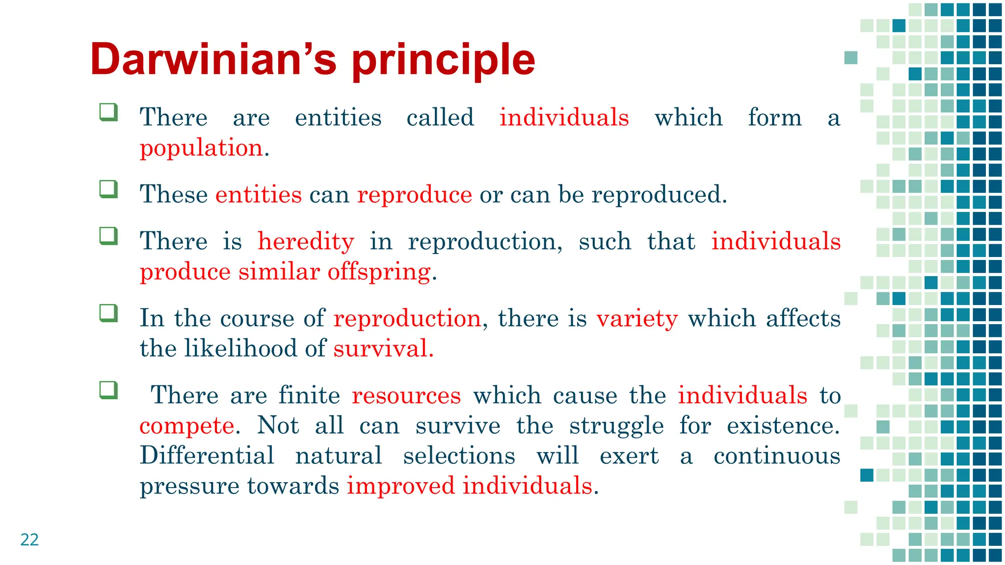
Darwinian’s principle
Thereare entities called individuals which form a
population.
These entities can reproduce or can be reproduced.
There is heredity in reproduction, such that individuals
produce similar offspring.
In the course of reproduction, there is variety which affects
the likelihood of survival.
There are finite resources which cause the individuals to
compete. Not all can survive the struggle for existence.
Differential natural selections will exert a continuous
pressure towards improved individuals.
22
23.
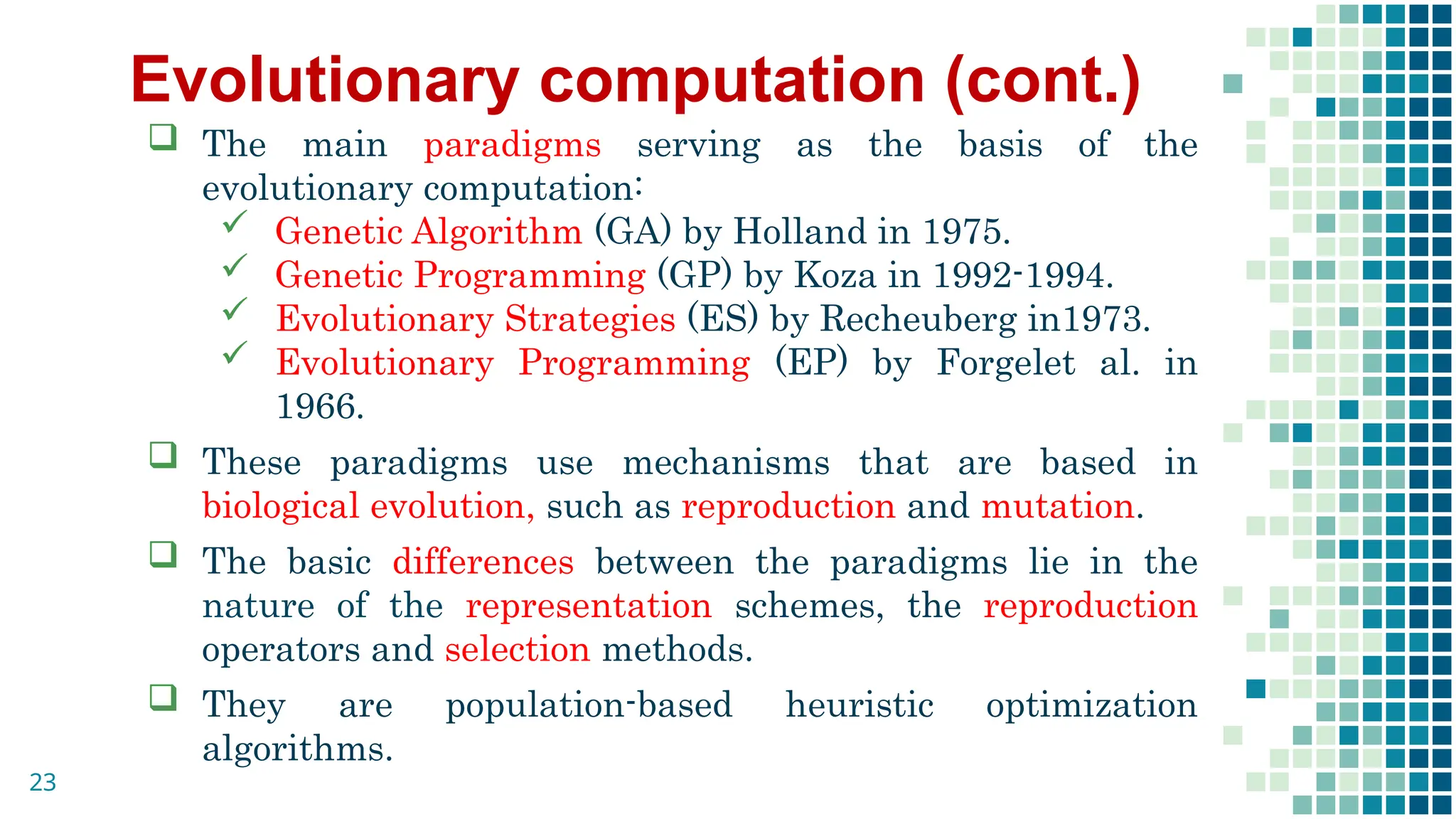
Evolutionary computation (cont.)
The main paradigms serving as the basis of the
evolutionary computation:
Genetic Algorithm (GA) by Holland in 1975.
Genetic Programming (GP) by Koza in 1992-1994.
Evolutionary Strategies (ES) by Recheuberg in1973.
Evolutionary Programming (EP) by Forgelet al. in
1966.
These paradigms use mechanisms that are based in
biological evolution, such as reproduction and mutation.
The basic differences between the paradigms lie in the
nature of the representation schemes, the reproduction
operators and selection methods.
They are population-based heuristic optimization
algorithms.
23
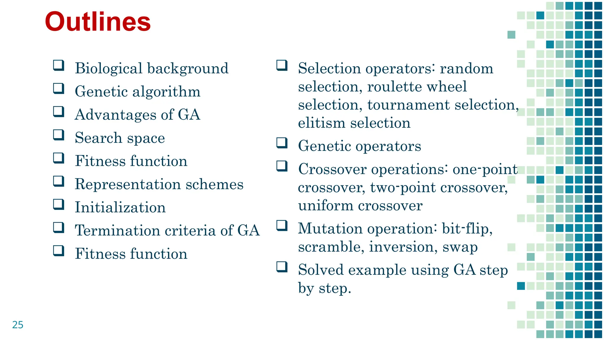
Outlines
Biological background
Genetic algorithm
Advantages of GA
Search space
Fitness function
Representation schemes
Initialization
Termination criteria of GA
Fitness function
Selection operators: random
selection, roulette wheel
selection, tournament selection,
elitism selection
Genetic operators
Crossover operations: one-point
crossover, two-point crossover,
uniform crossover
Mutation operation: bit-flip,
scramble, inversion, swap
Solved example using GA step
by step.
25
26.
Biological background
Thecell is the smallest structure
and functional unit of the
organism.
In the center of the cell, we have
nucleus which contains genome
containing 23 pair of
chromosomes.
The chromosome is made of DNA.
DNA is made of many genes. a
gene is a short section of DNA.
DNA has a twisted structure in
the shape of a double helix.
26
27.
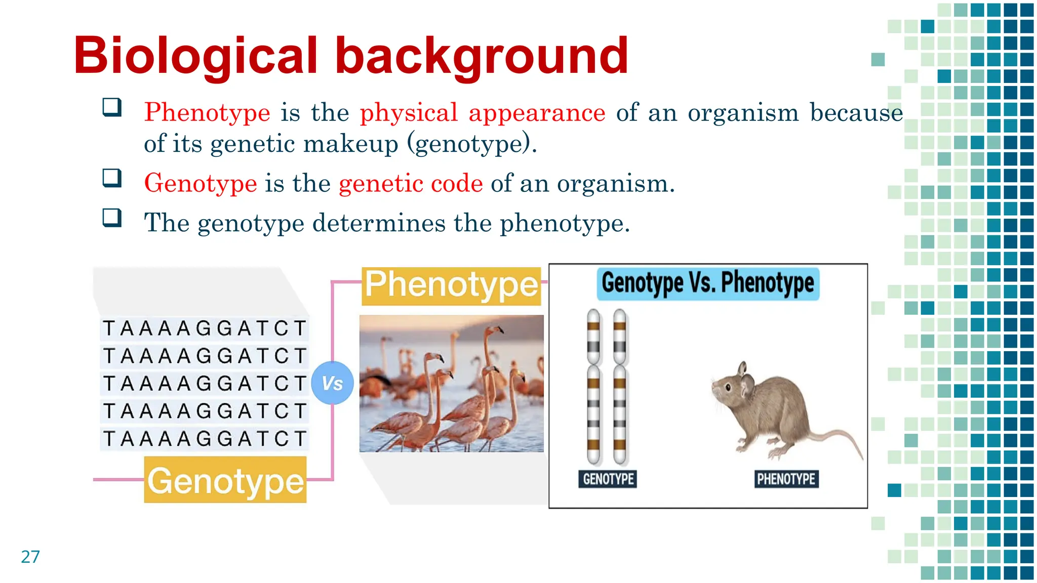
Biological background
Phenotypeis the physical appearance of an organism because
of its genetic makeup (genotype).
Genotype is the genetic code of an organism.
The genotype determines the phenotype.
27
28.
Genetic algorithm
Geneticalgorithm (GA) is a population-based probabilistic
search and optimization technique, which works based on
the mechanism of genetics and Darwin’s principle of
natural selection.
The GA was introduced by Prof. John Holland of the
University of Michigan, in 1965, although his seminal book
was published in 1975.
28
29.
Genetic algorithm(cont.)
29
Nature Geneticalgorithm
Environment Optimization problem
Individual living in this
environment
Feasible solutions
Individual degree of adaption to its
surrounding environment
Solution quality (fitness function)
A population of organisms A set of feasible solutions
Selection, recombination, mutation
in nature’s evolutionary process
Selection methods, crossover operator,
mutation operator
Evolution of populations to suit
their environment
Iteratively applying a set of genetic
operators on a set of feasible solutions
30.
Genetic algorithm
Initializea population with a random candidate chromosomes.
Repeat until termination criteria
Evaluate all chromosomes with a fitness function.
Select parents using one of selection methods.
Perform crossover operation with a probability Pc.
Perform mutation operation with a probability pm.
Replace the new population with the current population.
End termination criteria.
Return the best individual in the population.
30
Pseudocode of GA
31.
Advantages of GA
It is easy to understand.
It deals with complex real-world problems that the hard
computing techniques failed to solve.
It is modular, separate from application.
It is good for imprecise and noisy environments.
It supports multi-objective optimization.
It is easily distributed and parallelized.
31
32.
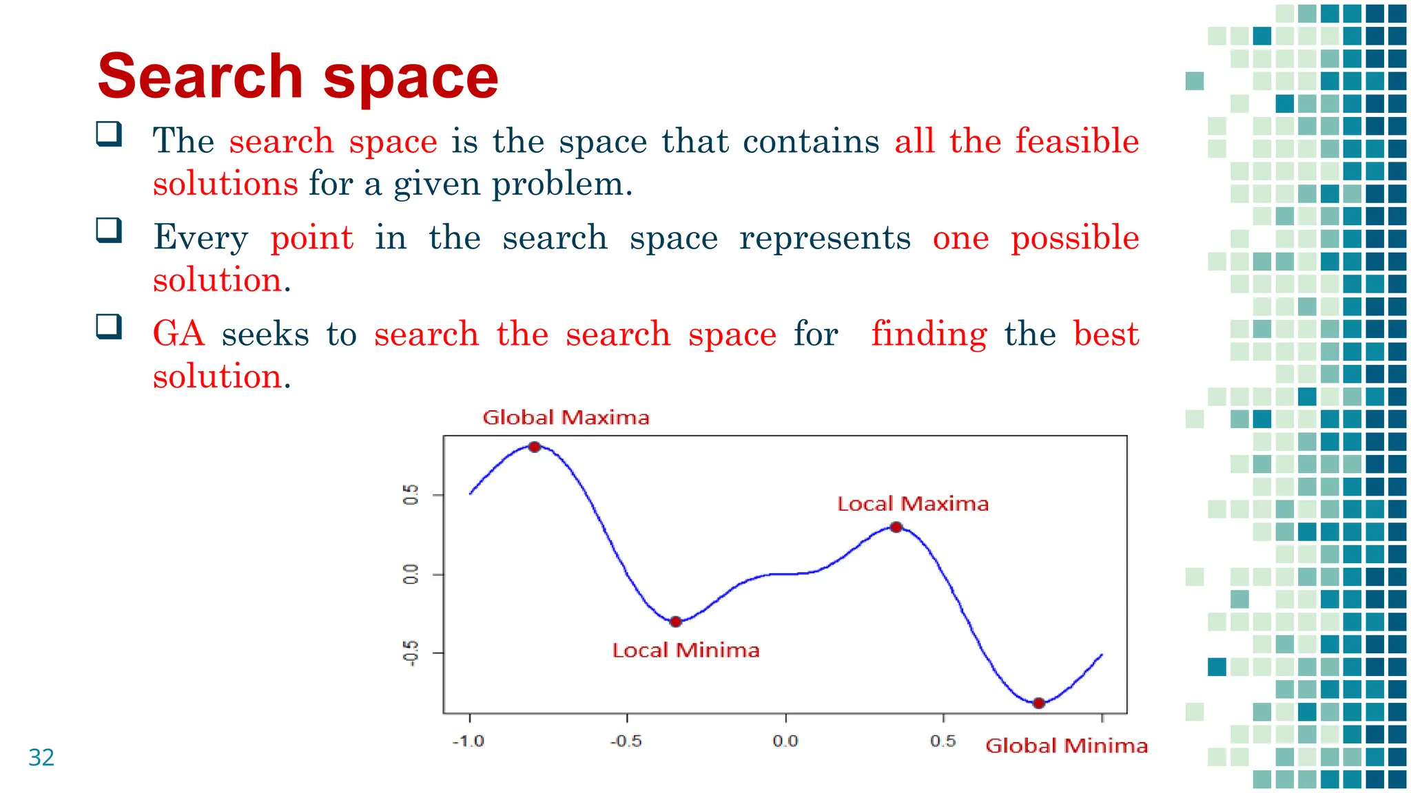
Search space
Thesearch space is the space that contains all the feasible
solutions for a given problem.
Every point in the search space represents one possible
solution.
GA seeks to search the search space for finding the best
solution.
32
33.
Representation schemes
Parametersof the solution (genes) are concatenated to form
a string (chromosome).
Encoding is a data structure for representing candidate
solutions.
Good encoding scheme may affect the performance of a GA.
Some genetic encoding schemes are:
Binary-encoding Simple GA or binary-coded GA
Real-valued encoding real-valued GA
Permutation encoding
33
Permutation encoding
Binary encoding Real-valued encoding
1 0 1 1 1.2 0.8 6.7 1.9 1 4 3 2
34.
Initialization
In thisstep, a population of N random individuals/
chromosomes are generated. N is the population size
(here, N=6).
G1 G2 G3 G4
Chromosome 1
Chromosome 2
Chromosome 3
Chromosome 4
Chromosome 5
Chromosome 6
34
35.
Termination criteria ofGA
The termination criteria can be:
Specified number of generations.
Specified number of fitness evaluations.
A minimum threshold reached.
No improvement in the best solutions for a specified
number of generations.
Memory/time constraints.
Combinations of above
35
36.
Fitness function
Afitness function is function which takes the solution as
input and produces the suitability of the solution as the
output.
It measures how good is a solution.
In some cases, the fitness function and the objective
function may be the same, while in others it might be
different based on the problem.
36
37.
Selection operators
Allthe candidate solutions or individuals contained in the
population may not be equally good in terms of their fitness
values calculated.
Selection operators are used to select the good ones from the
population of strings based on their fitness information.
Several selection operators have been developed:
Random selection
Proportionate selection/Roulette-wheel selection
Tournament selection
Elitism selection.
37
38.
Selective pressure
Eachselection operator is characterized by its selective
pressure.
A selection operator with a high selective pressure
decreases the diversity in population more rapidly than
a selection operator with a low selective pressure.
High selective pressure limits the exploration abilities
of the population.
38
39.
Random selection
Randomselection is the simplest selection operator.
Each individual has the same probability of 1/N to be
selected. N is the population size.
No fitness information is used, which means that the best
and the worst have exactly the same probability of
surviving to the next generations.
It has the lowest selective pressure among the selection
operators.
39
40.
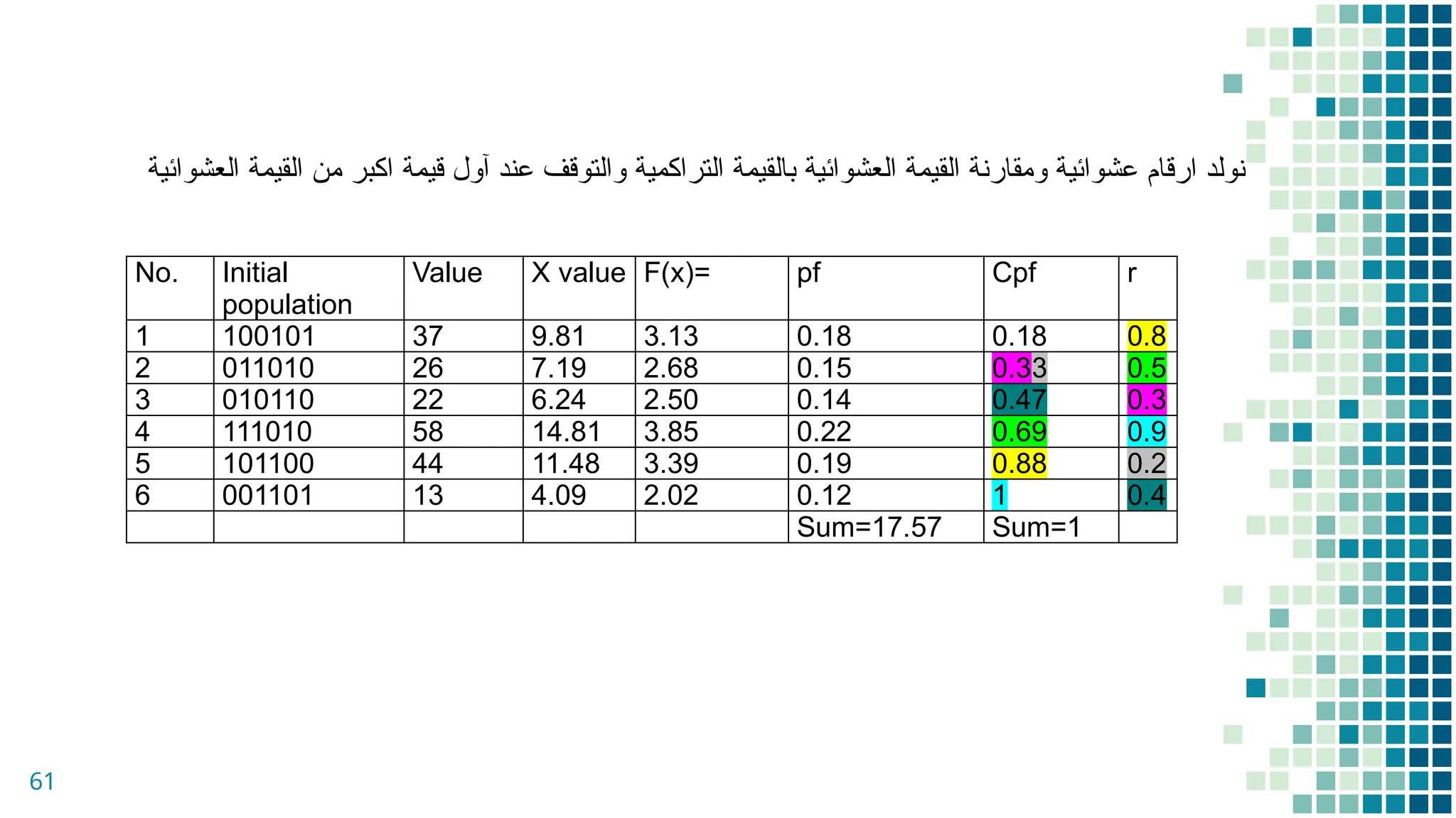
Roulette-wheel selection
Inthis operator, the probability of a chromosome for
being selected is proportional to its fitness.
It is implemented with the help of roulette wheel.
I works as follows:
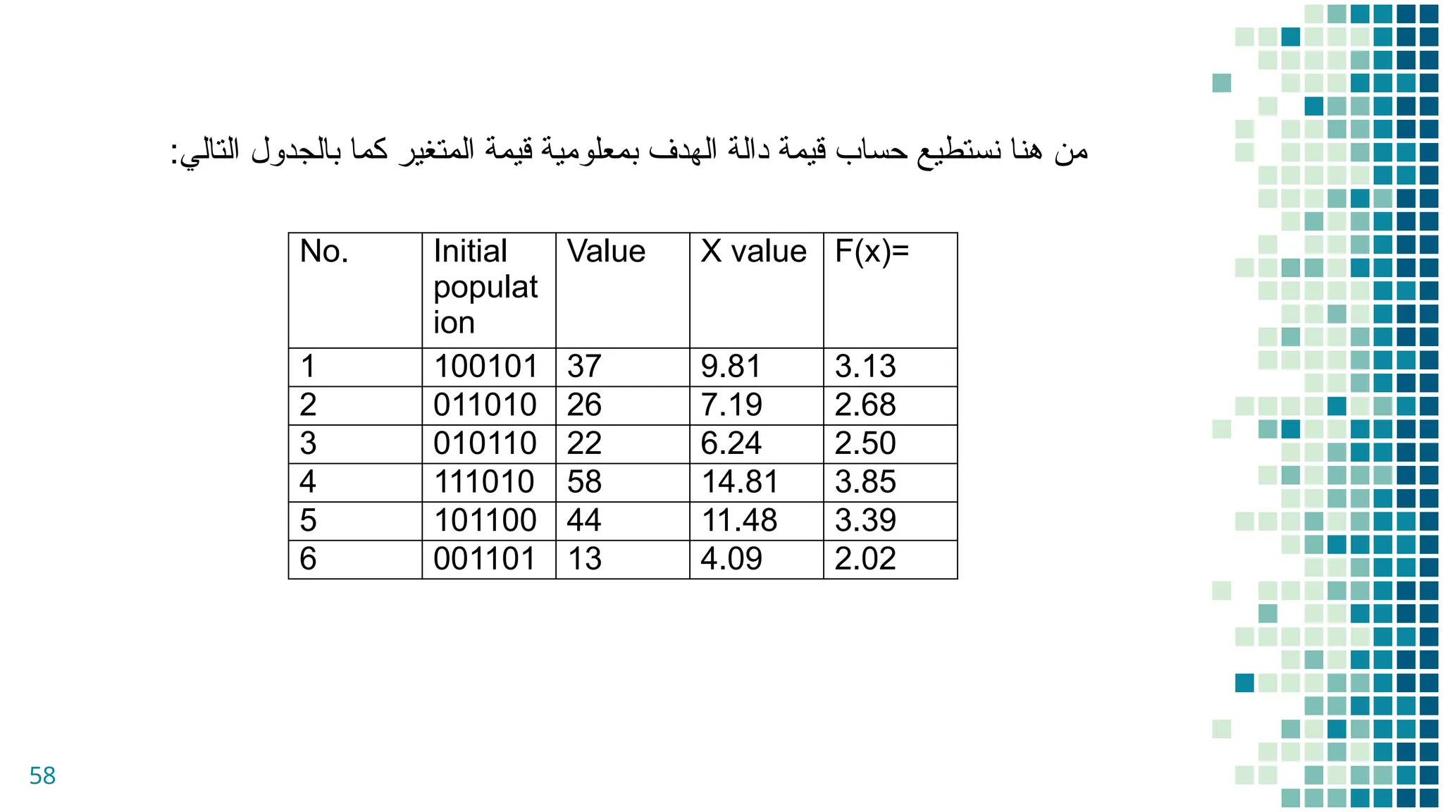
1. Calculate fitness of each chromosome ( ).
2. Divide the individual fitness by the whole population
fitness as follows:
,
3. N is the population size. is the proportional
fitness of an individual i.
4. Compute the cumulative proportional fitness of each
individual ( ).
40
1
( )
( )
( )
i
i N
i
i
f x
pf x
f x
1,...,
i N
( )
i
pf x
( )
i
f x
( )
i
cpf x
41.
Roulette-wheel selection (cont.)
5.Generate a random number (r) belonging to [0,1].
6. If , then select the i individual.
41
( )
i
cpf x
Because this selection is
directly proportional to its
fitness, it is possible that
strong individuals may
dominate in producing
offspring, thereby limiting the
diversity of the population.
In other words, it has a high
selective pressure.
Elitism selection
Elitismrefers to the process of ensuring that the best
individuals of the current population survive to the next
generation.
The best individuals are copied to the new population.
The more individuals that survive to the next generation,
the less the diversity of the new population.
43
44.
Tournament selection
Itselects randomly k individuals, where k is the size of
tournament group.
Then, the best individual is selected among the selected k
individuals.
44
Crossover operation
Inbiology, the most common form of recombination is
crossover.
Crossover is a process in which two parent
solutions/chromosomes are used to produce two new
offspring by replacing genes between the two parents.
The GA has a crossover probability that determines if
crossover will happen.
46
47.
one-point crossover
Inone-point crossover, a crossover point (p=2) is selected
and the tails of its two parents are swapped to generate
new offspring.
47
48.
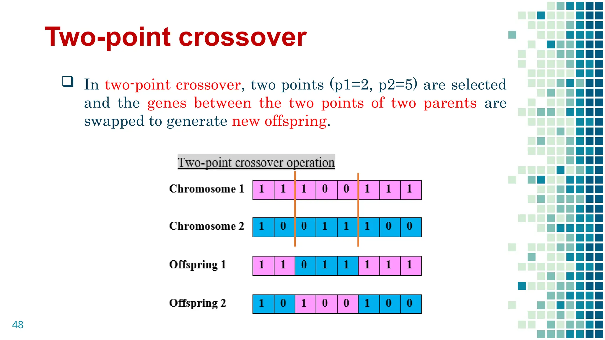
Two-point crossover
Intwo-point crossover, two points (p1=2, p2=5) are selected
and the genes between the two points of two parents are
swapped to generate new offspring.
48
49.
Uniform crossover
Ina uniform crossover, if a random number (r) is less than a
uniform probability (0.5), The new offspring is generated by
taking the genes from the first parent, otherwise, the genes
are taken from the second parent.
49
50.
Mutation operation
Mutationis a process in which the genes of one
chromosome are modified to generate a new chromosome.
The GA has a mutation probability that determines if
mutation will happen.
In bit-flip mutation one or more random bits are selected
to be flipped (01 or 10). This is used for binary
encoded GAs.
In swap mutation, we select two positions on the
chromosome at random, and interchange the values. This
is common in permutation encoding.
50
51.
Mutation operation
Scramblemutation is also popular with permutation
representations. From the entire chromosome, a subset of
genes is chosen, and their values are scrambled or shuffled
randomly.
In inversion mutation, we select a subset of genes like in
scramble mutation, but instead of shuffling the subset, we
invert the subset.
51
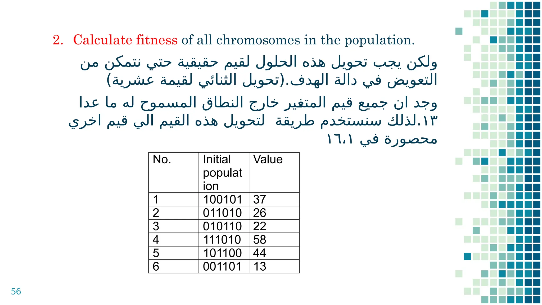
▪ Mapping thereal-valued numbers into real-valued in
range [1-16] using the linear mapping rule:
▪ L is number of bits
▪ D is the decoded value.
▪ 6
Then
▪ x1=1+=9.81
▪ x2=1+=7.19
57


![Roulette-wheel selection (cont.)
5. Generate a random number (r) belonging to [0,1].
6. If , then select the i individual.
41
( )
i
cpf x
Because this selection is
directly proportional to its
fitness, it is possible that
strong individuals may
dominate in producing
offspring, thereby limiting the
diversity of the population.
In other words, it has a high
selective pressure.](https://image.slidesharecdn.com/lec1-250909121144-710dc7d3/75/EVOLUTION-ALGORITHM-Optimization-pptx-41-2048.jpg)


![▪ Mapping the real-valued numbers into real-valued in
range [1-16] using the linear mapping rule:
▪ L is number of bits
▪ D is the decoded value.
▪ 6
Then
▪ x1=1+=9.81
▪ x2=1+=7.19
57](https://image.slidesharecdn.com/lec1-250909121144-710dc7d3/75/EVOLUTION-ALGORITHM-Optimization-pptx-57-2048.jpg)