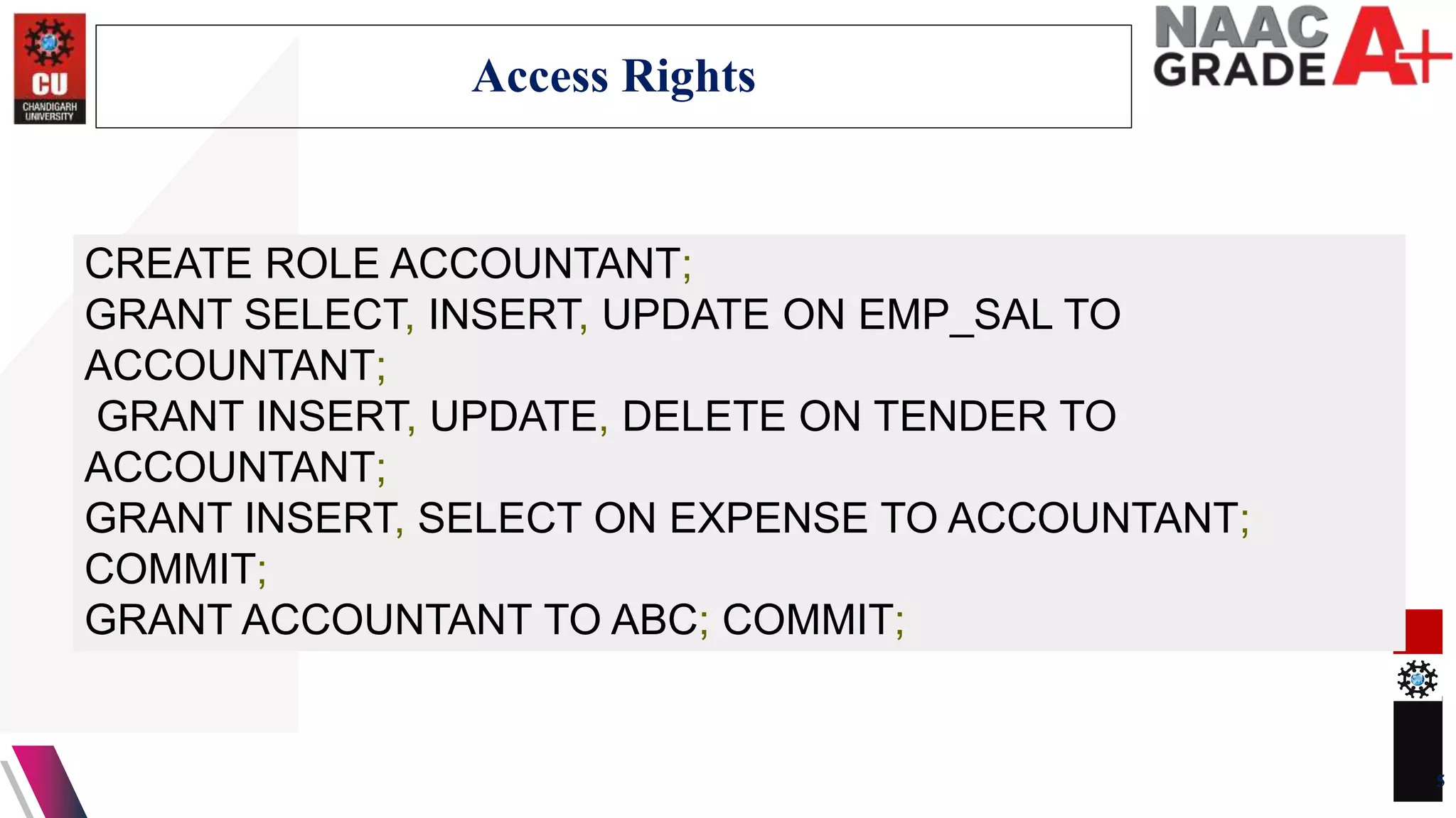
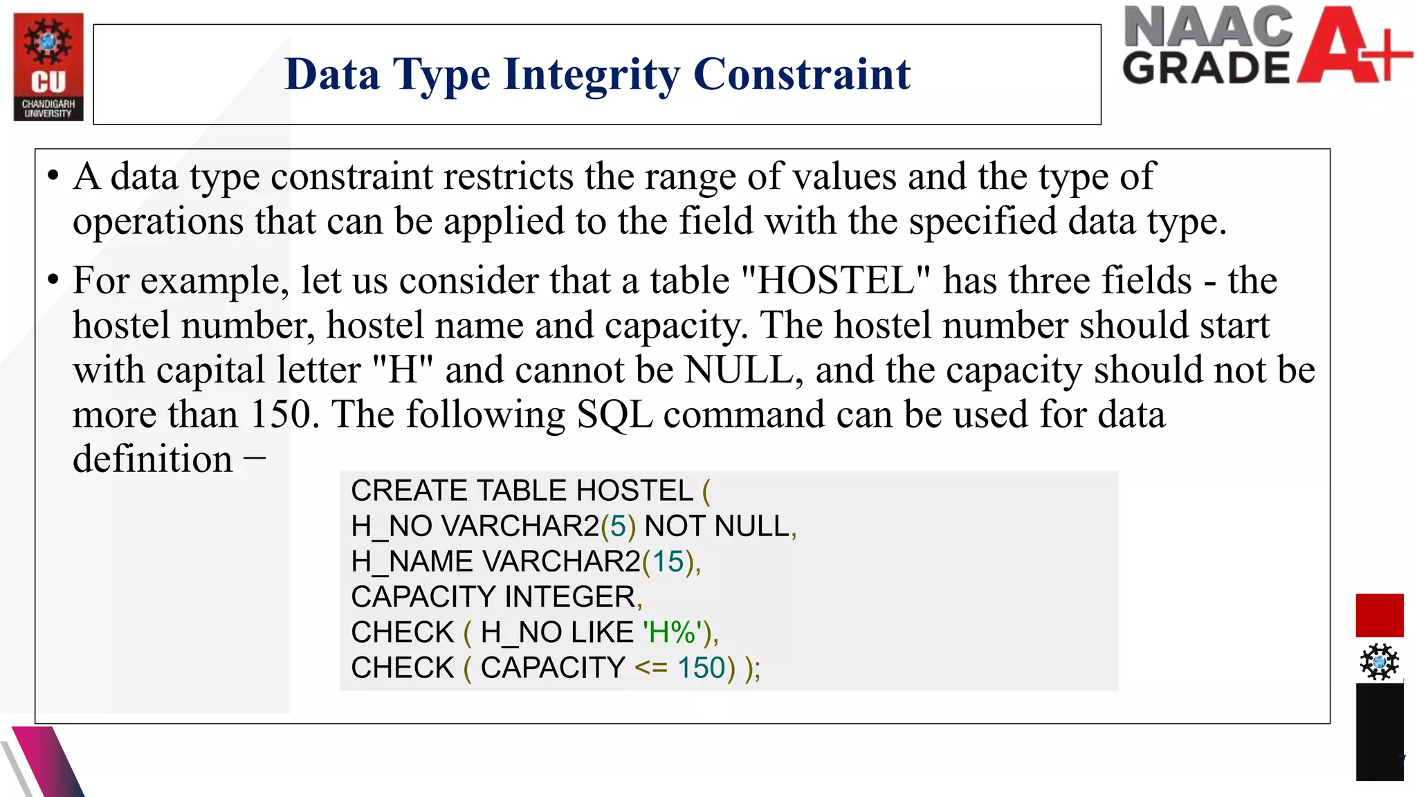
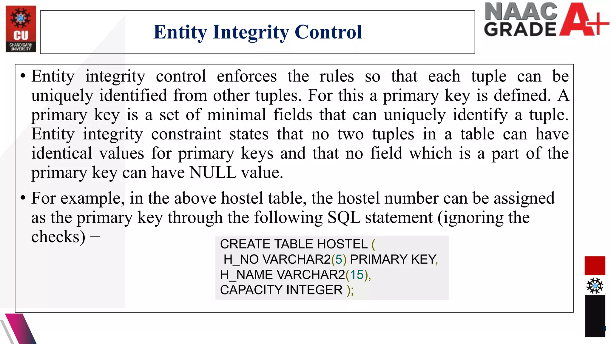
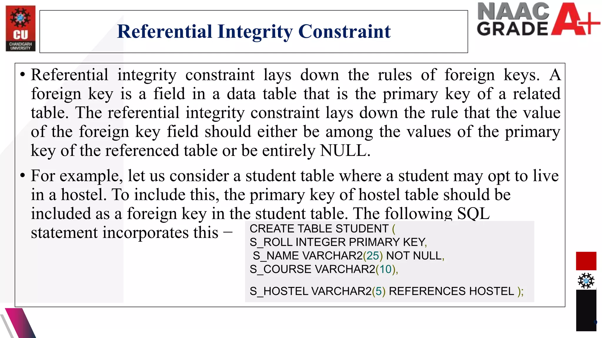
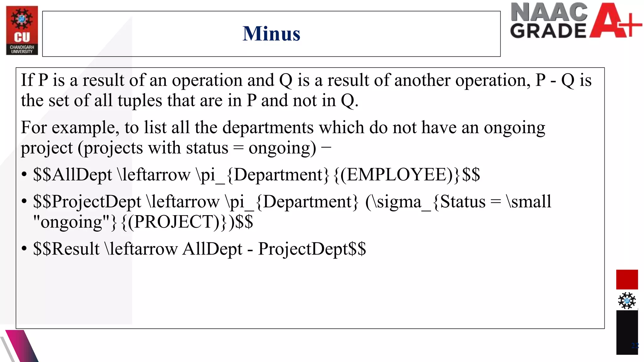
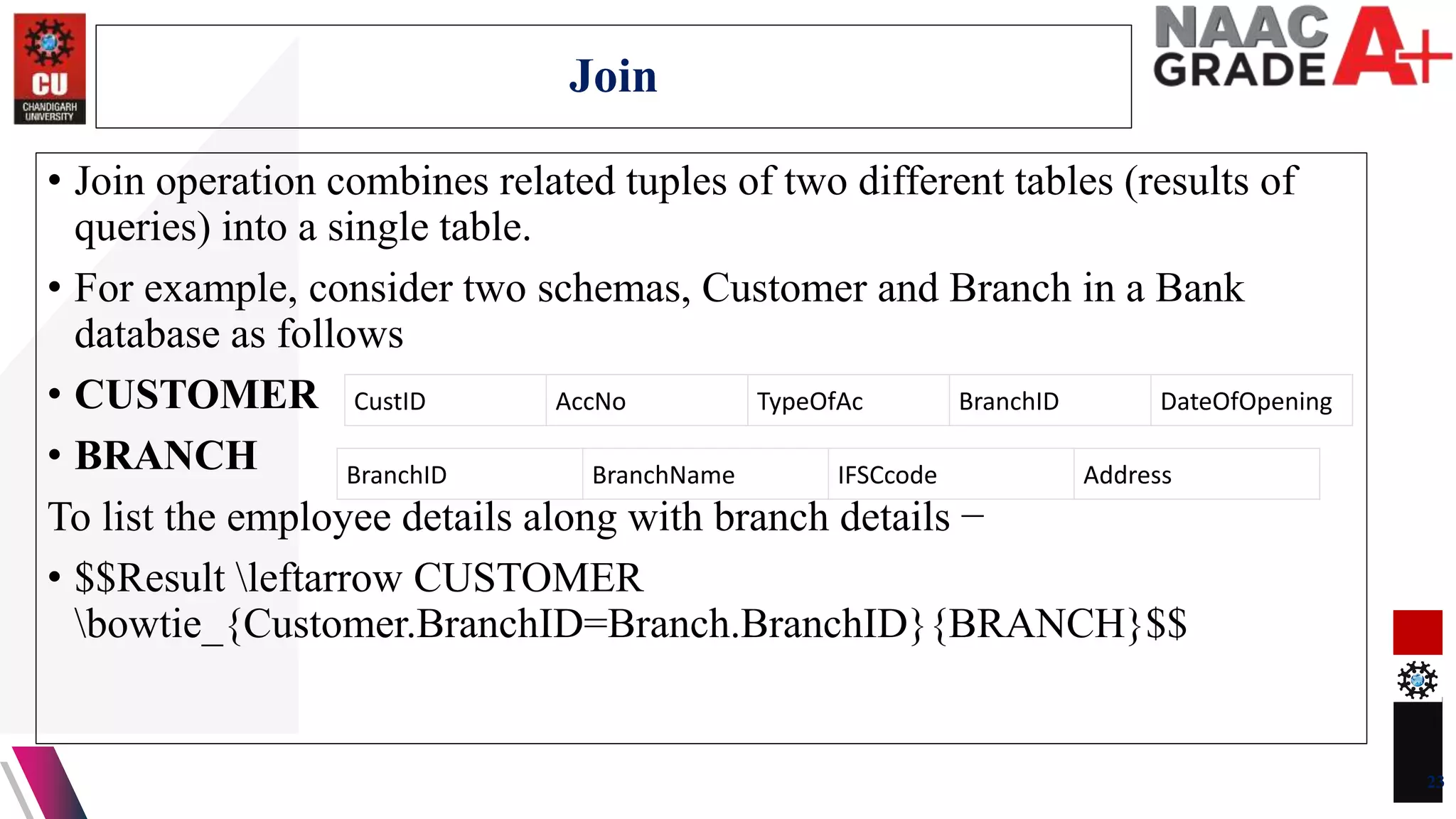
Database Terminology and DBLC.pptx

DISCOVER . LEARN . EMPOWER
UNIVERSITY INSTITUTE OF COMPUTING
MASTER OF COMPUTER APPLICATIONS
Advance Database Management System
1

• Database control refers to the task of enforcing regulations so as to provide
correct data to authentic users and applications of a database. In order that
correct data is available to users, all data should conform to the integrity
constraints defined in the database. Besides, data should be screened away
from unauthorized users so as to maintain security and privacy of the
database. Database control is one of the primary tasks of the database
administrator (DBA).
• The three dimensions of database control are −
• Authentication
• Access rights
• Integrity constraints
2
Database Control

• In a distributed database system, authentication is the process through
which only legitimate users can gain access to the data
resources.Authentication can be enforced in two levels −
• Controlling Access to Client Computer − At this level, user access is
restricted while login to the client computer that provides user-interface to
the database server. The most common method is a username/password
combination. However, more sophisticated methods like biometric
authentication may be used for high security data.
• Controlling Access to the Database Software − At this level, the database
software/administrator assigns some credentials to the user. The user gains
access to the database using these credentials. One of the methods is to
create a login account within the database server.
3
Authentication

• A user’s access rights refers to the privileges that the user is given
regarding DBMS operations such as the rights to create a table, drop a
table, add/delete/update tuples in a table or query upon the table.
• In distributed environments, since there are large number of tables and yet
larger number of users, it is not feasible to assign individual access rights
to users. So, DDBMS defines certain roles. A role is a construct with
certain privileges within a database system. Once the different roles are
defined, the individual users are assigned one of these roles. Often a
hierarchy of roles are defined according to the organization’s hierarchy of
authority and responsibility.
• For example, the following SQL statements create a role "Accountant" and
then assigns this role to user "ABC".
4
Access Rights

5
Access Rights
CREATE ROLE ACCOUNTANT;
GRANT SELECT, INSERT, UPDATE ON EMP_SAL TO
ACCOUNTANT;
GRANT INSERT, UPDATE, DELETE ON TENDER TO
ACCOUNTANT;
GRANT INSERT, SELECT ON EXPENSE TO ACCOUNTANT;
COMMIT;
GRANT ACCOUNTANT TO ABC; COMMIT;

Semantic integrity control defines and enforces the integrity constraints of
the database system.
• The integrity constraints are as follows −
• Data type integrity constraint
• Entity integrity constraint
• Referential integrity constraint
6
Semantic Integrity Control

• A data type constraint restricts the range of values and the type of
operations that can be applied to the field with the specified data type.
• For example, let us consider that a table "HOSTEL" has three fields - the
hostel number, hostel name and capacity. The hostel number should start
with capital letter "H" and cannot be NULL, and the capacity should not be
more than 150. The following SQL command can be used for data
definition −
7
Data Type Integrity Constraint
CREATE TABLE HOSTEL (
H_NO VARCHAR2(5) NOT NULL,
H_NAME VARCHAR2(15),
CAPACITY INTEGER,
CHECK ( H_NO LIKE 'H%'),
CHECK ( CAPACITY <= 150) );

• Entity integrity control enforces the rules so that each tuple can be
uniquely identified from other tuples. For this a primary key is defined. A
primary key is a set of minimal fields that can uniquely identify a tuple.
Entity integrity constraint states that no two tuples in a table can have
identical values for primary keys and that no field which is a part of the
primary key can have NULL value.
• For example, in the above hostel table, the hostel number can be assigned
as the primary key through the following SQL statement (ignoring the
checks) −
8
Entity Integrity Control
CREATE TABLE HOSTEL (
H_NO VARCHAR2(5) PRIMARY KEY,
H_NAME VARCHAR2(15),
CAPACITY INTEGER );

• Referential integrity constraint lays down the rules of foreign keys. A
foreign key is a field in a data table that is the primary key of a related
table. The referential integrity constraint lays down the rule that the value
of the foreign key field should either be among the values of the primary
key of the referenced table or be entirely NULL.
• For example, let us consider a student table where a student may opt to live
in a hostel. To include this, the primary key of hostel table should be
included as a foreign key in the student table. The following SQL
statement incorporates this −
9
Referential Integrity Constraint
CREATE TABLE STUDENT (
S_ROLL INTEGER PRIMARY KEY,
S_NAME VARCHAR2(25) NOT NULL,
S_COURSE VARCHAR2(10),
S_HOSTEL VARCHAR2(5) REFERENCES HOSTEL );

• When a query is placed, it is at first scanned, parsed and validated. An
internal representation of the query is then created such as a query tree or a
query graph. Then alternative execution strategies are devised for
retrieving results from the database tables. The process of choosing the
most appropriate execution strategy for query processing is called query
optimization.
10
Query Optimization

• In DDBMS, query optimization is a crucial task. The complexity is high
since number of alternative strategies may increase exponentially due to
the following factors −
• The presence of a number of fragments.
• Distribution of the fragments or tables across various sites.
• The speed of communication links.
• Disparity in local processing capabilities.
11
Query Optimization Issues in DDBMS

Hence, in a distributed system, the target is often to find a good execution
strategy for query processing rather than the best one. The time to execute a
query is the sum of the following −
• Time to communicate queries to databases.
• Time to execute local query fragments.
• Time to assemble data from different sites.
• Time to display results to the application.
12
Query Optimization Issues in DDBMS

• Query processing is a set of all activities starting from query placement to
displaying the results of the query. The steps are as shown in the following
diagram −
13
Query Processing

• Relational algebra defines the basic set of operations of relational database
model. A sequence of relational algebra operations forms a relational
algebra expression. The result of this expression represents the result of a
database query. The basic operations are −
• Projection
• Selection
• Union
• Intersection
• Minus
• Join
14
Relational Algebra

• Projection operation displays a subset of fields of a table. This gives a
vertical partition of the table. Syntax in Relational Algebra
• $$pi_{<{AttributeList}>}{(<{Table Name}>)}$$
• For example, let us consider the following Student database −
15
Projection
STUDENT
Roll_No Name Course Semester Gender
2 Amit Prasad BCA 1 Male
4 Varsha Tiwari BCA 1 Female
5 Asif Ali MCA 2 Male
6 Joe Wallace MCA 1 Male
8 Shivani Iyengar BCA 1 Female

• If we want to display the names and courses of all students, we will use the
following relational algebra expression −
• $$pi_{Name,Course}{(STUDENT)}$$
16
Projection

• Selection operation displays a subset of tuples of a table that satisfies
certain conditions. This gives a horizontal partition of the table. Syntax in
Relational Algebra
• $$sigma_{<{Conditions}>}{(<{Table Name}>)}$$
For example, in the Student table, if we want to display the details of all
students who have opted for MCA course, we will use the following
relational algebra expression −
• $$sigma_{Course} = {small "BCA"}^{(STUDENT)}$$
17
Selection

For most queries, we need a combination of projection and selection
operations. There are two ways to write these expressions −
• Using sequence of projection and selection operations.
• Using rename operation to generate intermediate results.
For example, to display names of all female students of the BCA course −
• Relational algebra expression using sequence of projection and selection
operations
• $$pi_{Name}(sigma_{Gender = small "Female" AND : Course = small
"BCA"}{(STUDENT)})$$
18
Combination of Projection and Selection
Operations

Relational algebra expression using rename operation to generate
intermediate results
• $$FemaleBCAStudent leftarrow sigma_{Gender = small "Female" AND
: Course = small "BCA"} {(STUDENT)}$$
• $$Result leftarrow pi_{Name}{(FemaleBCAStudent)}$$
19
Combination of Projection and Selection
Operations

If P is a result of an operation and Q is a result of another operation, the
union of P and Q ($p cup Q$) is the set of all tuples that is either in P or in
Q or in both without duplicates.
For example, to display all students who are either in Semester 1 or are in
BCA course −
• $$Sem1Student leftarrow sigma_{Semester = 1}{(STUDENT)}$$
• $$BCAStudent leftarrow sigma_{Course = small
"BCA"}{(STUDENT)}$$
• $$Result leftarrow Sem1Student cup BCAStudent$$
20
Union

• If P is a result of an operation and Q is a result of another operation, the
intersection of P and Q ( $p cap Q$ ) is the set of all tuples that are in P
and Q both.
• For example, given the following two schemas −
• EMPLOYEE
• PROJECT
To display the names of all cities where a project is located and also an
employee resides −
• $$CityEmp leftarrow pi_{City}{(EMPLOYEE)}$$
• $$CityProject leftarrow pi_{City}{(PROJECT)}$$
• $$Result leftarrow CityEmp cap CityProject$$
21
Intersection
EmpID Name City Department Salary
PId City Department Status

If P is a result of an operation and Q is a result of another operation, P - Q is
the set of all tuples that are in P and not in Q.
For example, to list all the departments which do not have an ongoing
project (projects with status = ongoing) −
• $$AllDept leftarrow pi_{Department}{(EMPLOYEE)}$$
• $$ProjectDept leftarrow pi_{Department} (sigma_{Status = small
"ongoing"}{(PROJECT)})$$
• $$Result leftarrow AllDept - ProjectDept$$
22
Minus

• Join operation combines related tuples of two different tables (results of
queries) into a single table.
• For example, consider two schemas, Customer and Branch in a Bank
database as follows
• CUSTOMER
• BRANCH
To list the employee details along with branch details −
• $$Result leftarrow CUSTOMER
bowtie_{Customer.BranchID=Branch.BranchID}{BRANCH}$$
23
Join
CustID AccNo TypeOfAc BranchID DateOfOpening
BranchID BranchName IFSCcode Address

• Data cleaning defines to clean the data by filling in the missing values,
smoothing noisy data, analyzing and removing outliers, and removing
inconsistencies in the data. Sometimes data at multiple levels of detail can
be different from what is required, for example, it can need the age ranges
of 20-30, 30-40, 40-50, and the imported data includes birth date. The data
can be cleans by splitting the data into appropriate types.
24
Data cleaning

Types of data cleaning
There are various types of data cleaning which are as follows −
• Missing Values − Missing values are filled with appropriate values. There
are the following approaches to fill the values.
• The tuple is ignored when it includes several attributes with missing values.
• The values are filled manually for the missing value.
• The same global constant can fill the values.
• The attribute mean can fill the missing values.
• The most probable value can fill the missing values.
25
Data cleaning

• Noisy data − Noise is a random error or variance in a measured variable.
There are the following smoothing methods to handle noise which are as
follows −
• Binning − These methods smooth out a arrange data value by consulting its
“neighborhood,” especially, the values around the noisy information. The arranged
values are distributed into multiple buckets or bins. Because binning methods
consult the neighborhood of values, they implement local smoothing.
• Regression − Data can be smoothed by fitting the information to a function,
including with regression. Linear regression contains finding the “best” line to fit
two attributes (or variables) so that one attribute can be used to forecast the other.
Multiple linear regression is a development of linear regression, where more than
two attributes are contained and the data are fit to a multidimensional area.
26
Data cleaning

• Clustering − Clustering supports in identifying the outliers. The same values are
organized into clusters and those values which fall outside the cluster are known as
outliers.
• Combined computer and human inspection − The outliers can also be recognized
with the support of computer and human inspection. The outliers pattern can be
descriptive or garbage. Patterns having astonishment value can be output to a list.
Inconsistence data − The inconsistency can be recorded in various
transactions, during data entry, or arising from integrating information from
multiple databases. Some redundancies can be recognized by correlation
analysis. Accurate and proper integration of the data from various sources
can decrease and avoid redundancy.
27
Data cleaning

Layers of Query Processing
Query processing has 4 layers:
• Query Decomposition
• Data Localization
• Global Query Optimization
• Distribution Query Execution
28
Layers of Query Processing

The first layer decomposes the calculus query into an algebraic query on
global relations. The information needed for this transformation is found in
the global conceptual schema describing the global relations.
Query decomposition can be viewed as four successive steps.
• Normalization
• Analysis
• Simplification
• Restructure
30
Query Decomposition

• First, the calculus query is rewritten in a normalized form that is suitable
for subsequent manipulation. Normalization of a query generally involves
the manipulation of the query quantifiers and of the query qualification by
applying logical operator priority.
• Second, the normalized query is analyzed semantically so that incorrect
queries are detected and rejected as early as possible. Techniques to detect
incorrect queries exist only for a subset of relational calculus. Typically, they
use some sort of graph that captures the semantics of the query.
31
Query Decomposition

• Third, the correct query (still expressed in relational calculus) is simplified.
One way to simplify a query is to eliminate redundant predicates. Note that
redundant queries are likely to arise when a query is the result of system
transformations applied to the user query. such transformations are used for
performing semantic data control (views, protection, and semantic integrity
control).
•Fourth, the calculus query is restructured as an algebraic query. The
traditional way to do this transformation toward a "“better" algebraic
specification is to start with an initial algebraic query and transform it in
order to find a "go
32
Query Decomposition

Query Processing Example
Query:
select salary from instructor where salary < 75000;
This query can be translated into either of the following relational-
algebra expressions:
•σsalary <75000(Πsalary (σsalary <75000(Πsalary ( instructor ))))
•Πsalary (σsalary <75000(Πsalary (σsalary <75000( instructor ))
33
Query Decomposition

• The input to the second layer is an algebraic query on global relations. The
main role of the second layer is to localize the query's data using data
distribution information in the fragment schema.
• This layer determines which fragments are involved in the query and
transforms the distributed query into a query on fragments.
• A global relation can be reconstructed by applying the fragmentation rules,
and then deriving a program, called a localization program, of relational
algebra operators, which then act on fragments.
34
Data Localization

Generating a query on fragments is done in two steps
• First, the query is mapped into a fragment query by substituting each
relation by its reconstruction program (also called materialization program).
• Second, the fragment query is simplified and restructured to produce
another "good" query.
35
Data Localization

• The input to the third layer is an algebraic query on fragments. The goal of
query optimization is to find an execution strategy for the query which is
close to optimal.
• The previous layers have already optimized the query, for example, by
eliminating redundant expressions. However, this optimization is
independent of fragment characteristics such as fragment allocation and
cardinalities.
• Query optimization consists of finding the "best" ordering of operators in
the query, including communication operators that minimize a cost function.
• The output of the query optimization layer is a optimized algebraic query
with communication operators included on fragments. It is typically
represented and saved (for future executions) as a distributed query
execution plan. 36
Global Query Optimization

• The last layer is performed by all the sites having fragments involved in the
query.
• Each sub query executing atone site, called a local query, is then
optimized using the local schema of the site and executed.
37
Distribution Query Execution

Database Terminology and DBLC.pptx

More Related Content

Similar to Database Terminology and DBLC.pptx

Recently uploaded

Database Terminology and DBLC.pptx