The document provides instructions for installing NumPy and Matplotlib on Ubuntu and includes examples of data creation, manipulation, and visualization using Python code. It covers creating one and two-dimensional arrays, performing basic mathematical operations, and generating plots for sine and cosine functions. Additionally, it demonstrates techniques for transforming and visualizing data, such as applying log transformations and displaying heatmaps.


![numpy arrays
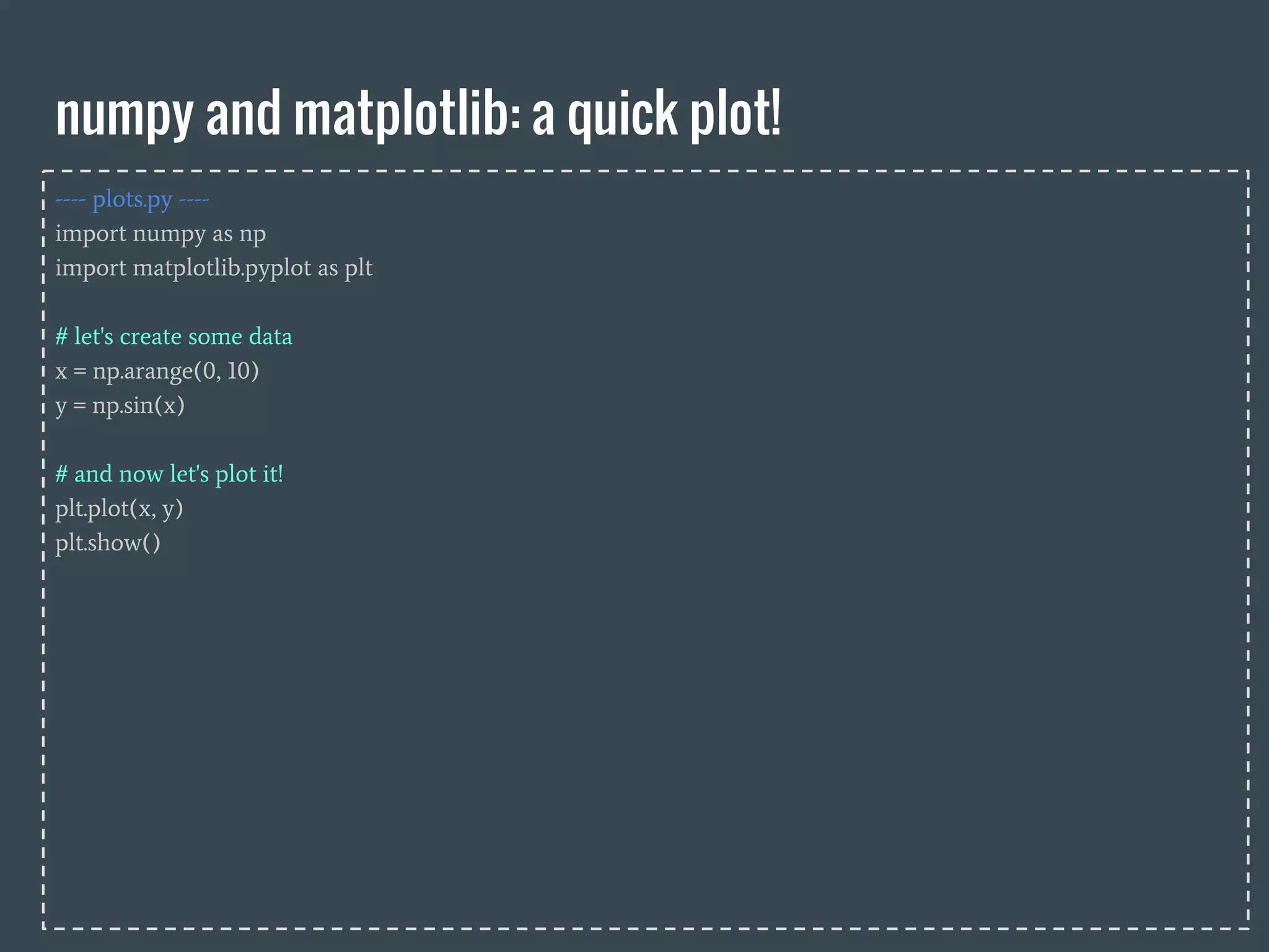
---- plots.py ----
import numpy as np
# creating an new empty 2-dimensional array/matrix:
a = np.zeros([3, 10])
# creating an new 2-dimensional matrix from array/lists:
a = np.array([[1,10,4],[3,9,2]])
# accessing array elements: indexes and slicing
print a.shape
# accessing array elements: indexes and slicing
print a[1,2] # row 1, element 2
print a[1] # row 1
print a[:,1] # column 1
print a[:,0:2] # remember that x:y selects x to y-1
A one-dimensional array:
a = np.array(list)
A two-dimensional array:
a = np.array(list-of-lists)
A two-dimensional array of zeros:
a = np.zeros([3, 10])](https://image.slidesharecdn.com/zyyw9t4vs06cq4bwtq1u-signature-8b30a4dc7f388ca820bf77ce8d424819e6bc869ded42016f2d1bbd7f84298e80-poli-160419081002/75/Class-8b-Numpy-Matplotlib-4-2048.jpg)
![numpy arrays
---- plots.py ----
import numpy as np
# creating an new 2-dimensional matrix from array/lists:
a = np.array([[1,10,4],[3,9,2]])
# changing a single values:
a[1,1] = 50
print a
# changing an entire column:
column = a[:,0]
a[:,1] = column
# basic math:
b = a[:,0] * 5
c = b + 9
# numpy math:
b = np.log10(a)
A single entry [row:col]
a[x:y]
A single row [row:col]
a[x,:]
A single column [row:col]
a[:,y]
see the full list of numpy mathfunctions:
http://docs.scipy.org/doc/numpy/reference/routines.math.html](https://image.slidesharecdn.com/zyyw9t4vs06cq4bwtq1u-signature-8b30a4dc7f388ca820bf77ce8d424819e6bc869ded42016f2d1bbd7f84298e80-poli-160419081002/75/Class-8b-Numpy-Matplotlib-5-2048.jpg)
![Heatmap!
Transpose an array:
data = data.transpose()
absolute value of matrix:
data = np.abs(data)
log10 of a matrix:
data = np.log10(data)
1. Read the matrix from the file (use np.loadtxt(“data.txt”))
2. Transpose the matrix
3. Apply a log10 transformation to all values
4. Copy row 11 to 15 and 18 (start counting at zero) (don’t forget n -1!)
5. Copy column 8 to columns 9 to 11 (start counting at zero) (don’t forget n -1!)
6. Transform all numbers to positive
7. Multiply all numbers between coordinates (2,3) and (18,7) by 20
8. Display the final result as a heatmap. It should be obvious if you got it right :P .
displaying a heatmap:
plt.pcolor(data)
plt.show()
selecting value, rows, columns...
data[x:y] (value)
data[x,:] (row)
data[:,y] (column)](https://image.slidesharecdn.com/zyyw9t4vs06cq4bwtq1u-signature-8b30a4dc7f388ca820bf77ce8d424819e6bc869ded42016f2d1bbd7f84298e80-poli-160419081002/75/Class-8b-Numpy-Matplotlib-6-2048.jpg)
![making plots just a little prettier!
---- plots.py ----
import numpy as np
import matplotlib.pyplot as plt
# Compute the x and y coordinates for points on sine and cosine curves
x = np.arange(0, 3 * np.pi, 0.1)
y_sin = np.sin(x)
y_cos = np.cos(x)
# Plot the points using matplotlib
plt.plot(x, y_sin)
plt.plot(x, y_cos)
plt.xlabel('x axis label')
plt.ylabel('y axis label')
plt.title('Sine and Cosine')
plt.legend(['Sine', 'Cosine'])
plt.show()](https://image.slidesharecdn.com/zyyw9t4vs06cq4bwtq1u-signature-8b30a4dc7f388ca820bf77ce8d424819e6bc869ded42016f2d1bbd7f84298e80-poli-160419081002/75/Class-8b-Numpy-Matplotlib-7-2048.jpg)


![NUMPY [Autosaved] .pptx](https://cdn.slidesharecdn.com/ss_thumbnails/numpyautosaved-240106041504-989a0cc3-thumbnail.jpg?width=640&height=640&fit=bounds)