Downloaded 90 times


![Message Passing Systems
8
Google’s Pregel [SIGMOD’10]
»Think like a vertex
»Message passing
»Iterative
• Superstep](https://image.slidesharecdn.com/sigmod16tutorial-160706202924/75/Big-Graph-Analytics-Systems-Sigmod16-Tutorial-8-2048.jpg)
![Message Passing Systems
9
Google’s Pregel [SIGMOD’10]
»Vertex Partitioning
0
1 2
3
4 5 6
7 8
0 1 3 1 0 2 3 2 1 3 4 7
3 0 1 2 7 4 2 5 7 5 4 6
6 5 8 7 2 3 4 8 8 6 7
M0 M1 M2](https://image.slidesharecdn.com/sigmod16tutorial-160706202924/75/Big-Graph-Analytics-Systems-Sigmod16-Tutorial-9-2048.jpg)
![Message Passing Systems
10
Google’s Pregel [SIGMOD’10]
»Programming Interface
• u.compute(msgs)
• u.send_msg(v, msg)
• get_superstep_number()
• u.vote_to_halt()
Called inside u.compute(msgs)](https://image.slidesharecdn.com/sigmod16tutorial-160706202924/75/Big-Graph-Analytics-Systems-Sigmod16-Tutorial-10-2048.jpg)
![Message Passing Systems
11
Google’s Pregel [SIGMOD’10]
»Vertex States
• Active / inactive
• Reactivated by messages
»Stop Condition
• All vertices halted, and
• No pending messages](https://image.slidesharecdn.com/sigmod16tutorial-160706202924/75/Big-Graph-Analytics-Systems-Sigmod16-Tutorial-11-2048.jpg)
![Message Passing Systems
12
Google’s Pregel [SIGMOD’10]
»Hash-Min: Connected Components
7
0
1
2
3
4
5 67 8
0 6 85
2
4
1
3
Superstep 1](https://image.slidesharecdn.com/sigmod16tutorial-160706202924/75/Big-Graph-Analytics-Systems-Sigmod16-Tutorial-12-2048.jpg)
![Message Passing Systems
13
Google’s Pregel [SIGMOD’10]
»Hash-Min: Connected Components
5
0
1
2
3
4
5 67 8
0 0 60
0
2
0
1
Superstep 2](https://image.slidesharecdn.com/sigmod16tutorial-160706202924/75/Big-Graph-Analytics-Systems-Sigmod16-Tutorial-13-2048.jpg)
![Message Passing Systems
14
Google’s Pregel [SIGMOD’10]
»Hash-Min: Connected Components
0
0
1
2
3
4
5 67 8
0 0 00
0
0
0
0
Superstep 3](https://image.slidesharecdn.com/sigmod16tutorial-160706202924/75/Big-Graph-Analytics-Systems-Sigmod16-Tutorial-14-2048.jpg)
![Message Passing Systems
15
Practical Pregel Algorithm (PPA) [PVLDB’14]
»First cost model for Pregel algorithm design
»PPAs for fundamental graph problems
• Breadth-first search
• List ranking
• Spanning tree
• Euler tour
• Pre/post-order traversal
• Connected components
• Bi-connected components
• Strongly connected components
• ...](https://image.slidesharecdn.com/sigmod16tutorial-160706202924/75/Big-Graph-Analytics-Systems-Sigmod16-Tutorial-15-2048.jpg)
![Message Passing Systems
16
Practical Pregel Algorithm (PPA) [PVLDB’14]
»Linear cost per superstep
• O(|V| + |E|) message number
• O(|V| + |E|) computation time
• O(|V| + |E|) memory space
»Logarithm number of supersteps
• O(log |V|) supersteps
O(log|V|) = O(log|E|)
How about load balancing?](https://image.slidesharecdn.com/sigmod16tutorial-160706202924/75/Big-Graph-Analytics-Systems-Sigmod16-Tutorial-16-2048.jpg)
![Message Passing Systems
17
Balanced PPA (BPPA) [PVLDB’14]
»din(v): in-degree of v
»dout(v): out-degree of v
»Linear cost per superstep
• O(din(v) + dout(v)) message number
• O(din(v) + dout(v)) computation time
• O(din(v) + dout(v)) memory space
»Logarithm number of supersteps](https://image.slidesharecdn.com/sigmod16tutorial-160706202924/75/Big-Graph-Analytics-Systems-Sigmod16-Tutorial-17-2048.jpg)
![Message Passing Systems
18
BPPA Example: List Ranking [PVLDB’14]
»A basic operation of Euler tour technique
»Linked list where each element v has
• Value val(v)
• Predecessor pred(v)
»Element at the head has pred(v) = NULL
11111NULL
v1 v2 v3 v4 v5
Toy Example: val(v) = 1 for all v](https://image.slidesharecdn.com/sigmod16tutorial-160706202924/75/Big-Graph-Analytics-Systems-Sigmod16-Tutorial-18-2048.jpg)
![Message Passing Systems
19
BPPA Example: List Ranking [PVLDB’14]
»Compute sum(v) for each element v
• Summing val(v) and values of all predecessors
»WhyTeraSort cannot work?
54321NULL
v1 v2 v3 v4 v5](https://image.slidesharecdn.com/sigmod16tutorial-160706202924/75/Big-Graph-Analytics-Systems-Sigmod16-Tutorial-19-2048.jpg)
![Message Passing Systems
20
BPPA Example: List Ranking [PVLDB’14]
»Pointer jumping / path doubling
• sum(v) ← sum(v) + sum(pred(v))
• pred(v) ← pred(pred(v))
11111NULL
v1 v2 v3 v4 v5
As long as pred(v) ≠ NULL](https://image.slidesharecdn.com/sigmod16tutorial-160706202924/75/Big-Graph-Analytics-Systems-Sigmod16-Tutorial-20-2048.jpg)
![Message Passing Systems
21
BPPA Example: List Ranking [PVLDB’14]
»Pointer jumping / path doubling
• sum(v) ← sum(v) + sum(pred(v))
• pred(v) ← pred(pred(v))
11111NULL
22221NULL
v1 v2 v3 v4 v5](https://image.slidesharecdn.com/sigmod16tutorial-160706202924/75/Big-Graph-Analytics-Systems-Sigmod16-Tutorial-21-2048.jpg)
![Message Passing Systems
22
BPPA Example: List Ranking [PVLDB’14]
»Pointer jumping / path doubling
• sum(v) ← sum(v) + sum(pred(v))
• pred(v) ← pred(pred(v))
NULL
22221NULL
44321NULL
v1 v2 v3 v4 v5
11111](https://image.slidesharecdn.com/sigmod16tutorial-160706202924/75/Big-Graph-Analytics-Systems-Sigmod16-Tutorial-22-2048.jpg)
![Message Passing Systems
23
BPPA Example: List Ranking [PVLDB’14]
»Pointer jumping / path doubling
• sum(v) ← sum(v) + sum(pred(v))
• pred(v) ← pred(pred(v))
NULL
22221NULL
44321NULL
54321NULL
v1 v2 v3 v4 v5
11111
O(log |V|) supersteps](https://image.slidesharecdn.com/sigmod16tutorial-160706202924/75/Big-Graph-Analytics-Systems-Sigmod16-Tutorial-23-2048.jpg)


![Message Passing Systems
34
Pregel+ [WWW’15]
»Vertex Mirroring
»Request-Respond Paradigm](https://image.slidesharecdn.com/sigmod16tutorial-160706202924/75/Big-Graph-Analytics-Systems-Sigmod16-Tutorial-34-2048.jpg)
![Message Passing Systems
35
Pregel+ [WWW’15]
»Vertex Mirroring
M3
w1
w2
wk
……
M2
v1
v2
vj
……
M1
u1
u2
ui
……
…
…](https://image.slidesharecdn.com/sigmod16tutorial-160706202924/75/Big-Graph-Analytics-Systems-Sigmod16-Tutorial-35-2048.jpg)
![Message Passing Systems
36
Pregel+ [WWW’15]
»Vertex Mirroring
M3
w1
w2
wk
……
M2
v1
v2
vj
……
M1
u1
u2
ui
……
uiui
…
…](https://image.slidesharecdn.com/sigmod16tutorial-160706202924/75/Big-Graph-Analytics-Systems-Sigmod16-Tutorial-36-2048.jpg)
![Message Passing Systems
37
Pregel+ [WWW’15]
»Vertex Mirroring: Create mirror for u4?
M1
u1
u4
…
v1 v2
v4v1 v2 v3
u2 v1 v2
u3 v1 v2
M2
v1
v4
…
v2
v3](https://image.slidesharecdn.com/sigmod16tutorial-160706202924/75/Big-Graph-Analytics-Systems-Sigmod16-Tutorial-37-2048.jpg)
![Message Passing Systems
38
Pregel+ [WWW’15]
»Vertex Mirroring v.s. Message Combining
M1
u1
u4
…
v1 v2
v4v1 v2 v3
u2 v1 v2
u3 v1 v2
M1
u1
u4
…
u2
u3
M2
v1
v4
…
v2
v3
a(u1) + a(u2)
+ a(u3) + a(u4)](https://image.slidesharecdn.com/sigmod16tutorial-160706202924/75/Big-Graph-Analytics-Systems-Sigmod16-Tutorial-38-2048.jpg)
![Message Passing Systems
39
Pregel+ [WWW’15]
»Vertex Mirroring v.s. Message Combining
M1
u1
u4
…
v1 v2
v4v1 v2 v3
u2 v1 v2
u3 v1 v2
M1
u1
u4
…
u2
u3
M2
v1
v4
…
v2
v3
u4
a(u1) + a(u2) + a(u3)
a(u4)](https://image.slidesharecdn.com/sigmod16tutorial-160706202924/75/Big-Graph-Analytics-Systems-Sigmod16-Tutorial-39-2048.jpg)
![Message Passing Systems
40
Pregel+ [WWW’15]
»Vertex Mirroring: Only mirror high-degree vertices
»Choice of degree threshold τ
• M machines, n vertices, m edges
• Average degree: degavg = m / n
• Optimal τ is M · exp{degavg / M}](https://image.slidesharecdn.com/sigmod16tutorial-160706202924/75/Big-Graph-Analytics-Systems-Sigmod16-Tutorial-40-2048.jpg)
![Message Passing Systems
41
Pregel+ [WWW’15]
» Request-Respond Paradigm
v1
v4
v2
v3
u
M1
a(u)
M2
<v1>
<v2>
<v3>
<v4>](https://image.slidesharecdn.com/sigmod16tutorial-160706202924/75/Big-Graph-Analytics-Systems-Sigmod16-Tutorial-41-2048.jpg)
![Message Passing Systems
42
Pregel+ [WWW’15]
» Request-Respond Paradigm
v1
v4
v2
v3
u
M1
a(u)
M2
a(u)
a(u)
a(u)
a(u)](https://image.slidesharecdn.com/sigmod16tutorial-160706202924/75/Big-Graph-Analytics-Systems-Sigmod16-Tutorial-42-2048.jpg)
![Message Passing Systems
43
Pregel+ [WWW’15]
»A vertex v can request attribute a(u) in superstep i
» a(u) will be available in superstep (i + 1)](https://image.slidesharecdn.com/sigmod16tutorial-160706202924/75/Big-Graph-Analytics-Systems-Sigmod16-Tutorial-43-2048.jpg)
![Message Passing Systems
44
v1
v4
v2
v3
u
M1
D[u]
M2
request u
u | D[u]
Pregel+ [WWW’15]
»A vertex v can request attribute a(u) in superstep I
» a(u) will be available in superstep (i + 1)](https://image.slidesharecdn.com/sigmod16tutorial-160706202924/75/Big-Graph-Analytics-Systems-Sigmod16-Tutorial-44-2048.jpg)

![Message Passing Systems
46
Vertex Migration
»WindCatch [ICDE’13]
• Runtime improved by 31.5% for PageRank (best)
• 2% for shortest path computation
• 9% for maximal matching
»Stanford’s GPS [SSDBM’13]
»Mizan [EuroSys’13]
• Hash-based and METIS partitioning: no improvement
• Range-based partitioning: around 40% improvement](https://image.slidesharecdn.com/sigmod16tutorial-160706202924/75/Big-Graph-Analytics-Systems-Sigmod16-Tutorial-46-2048.jpg)
![Message Passing Systems
Dynamic Concurrency Control
»PAGE [TKDE’15]
• Better partitioning → slower ?
47](https://image.slidesharecdn.com/sigmod16tutorial-160706202924/75/Big-Graph-Analytics-Systems-Sigmod16-Tutorial-47-2048.jpg)
![Message Passing Systems
Dynamic Concurrency Control
»PAGE [TKDE’15]
• Message generation
• Local message processing
• Remote message processing
48](https://image.slidesharecdn.com/sigmod16tutorial-160706202924/75/Big-Graph-Analytics-Systems-Sigmod16-Tutorial-48-2048.jpg)
![Message Passing Systems
Dynamic Concurrency Control
»PAGE [TKDE’15]
• Monitors speeds of the 3 operations
• Dynamically adjusts number of threads for the 3 operations
• Criteria
- Speed of message processing = speed of incoming messages
- Thread numbers for local & remote message processing are
proportional to speed of local & remote message processing
49](https://image.slidesharecdn.com/sigmod16tutorial-160706202924/75/Big-Graph-Analytics-Systems-Sigmod16-Tutorial-49-2048.jpg)
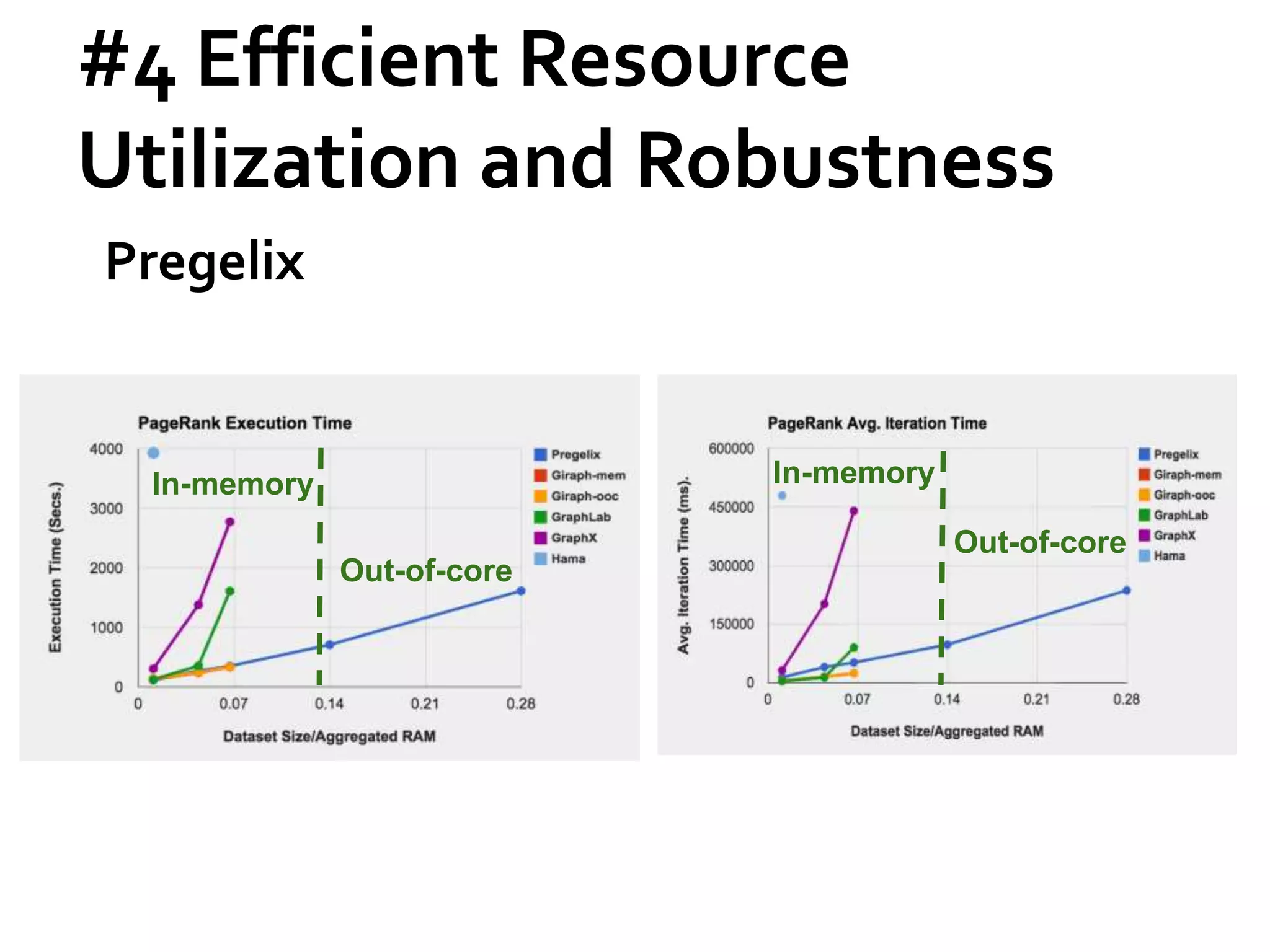
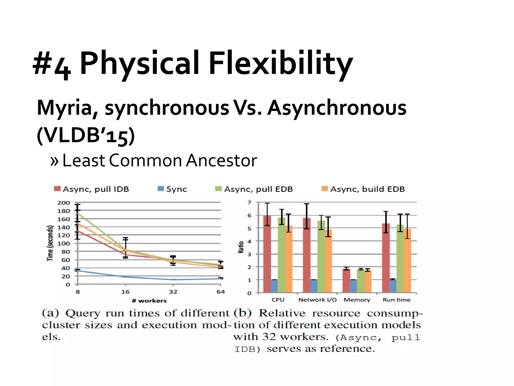
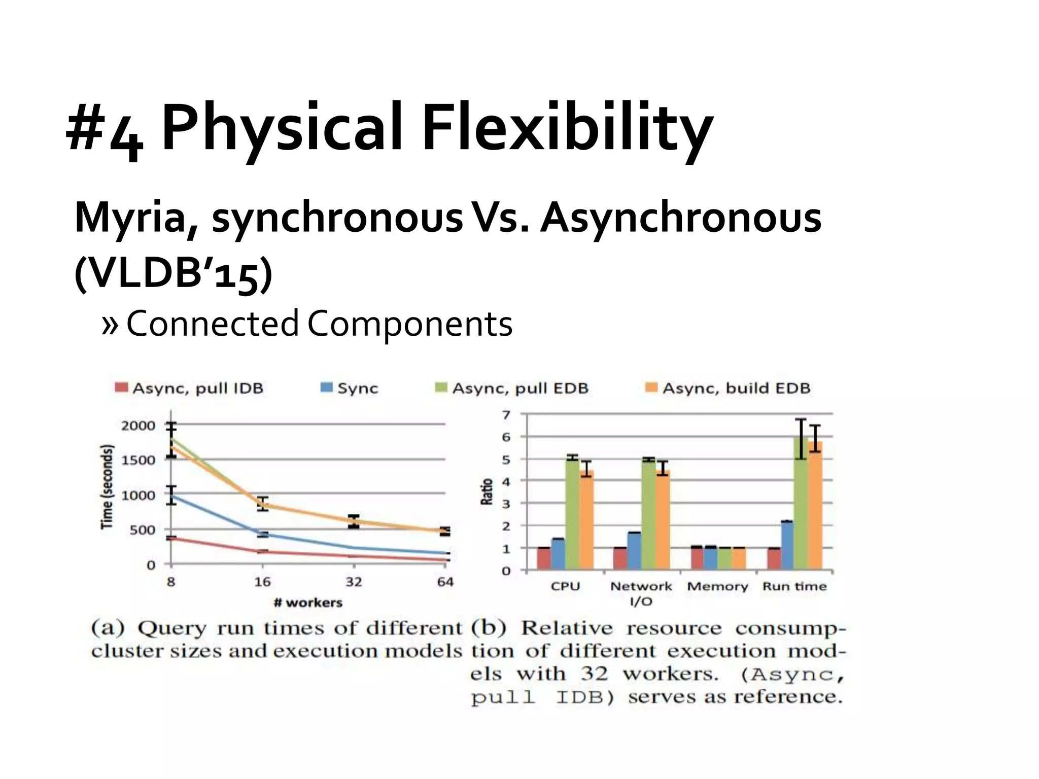
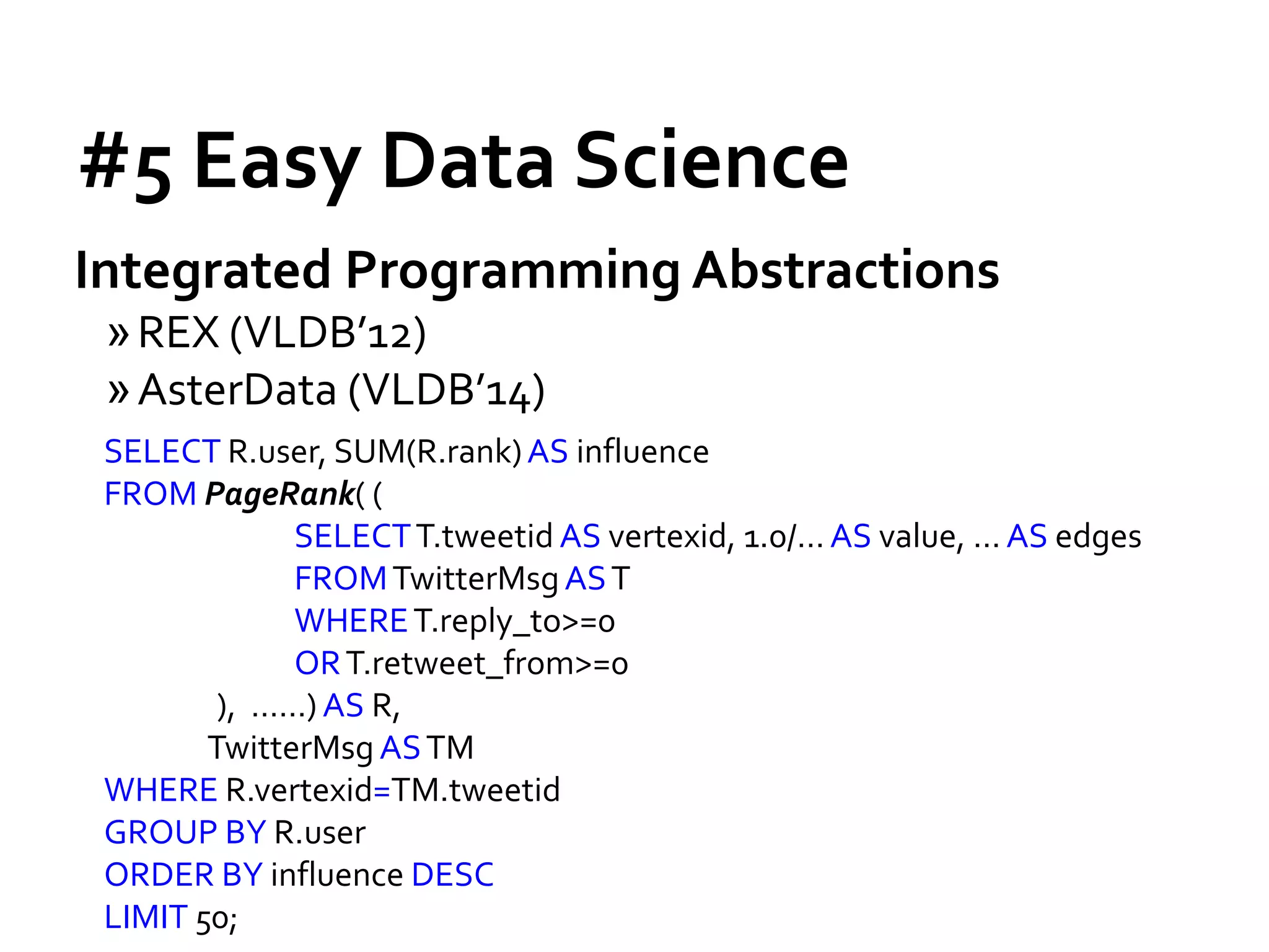
![Message Passing Systems
51
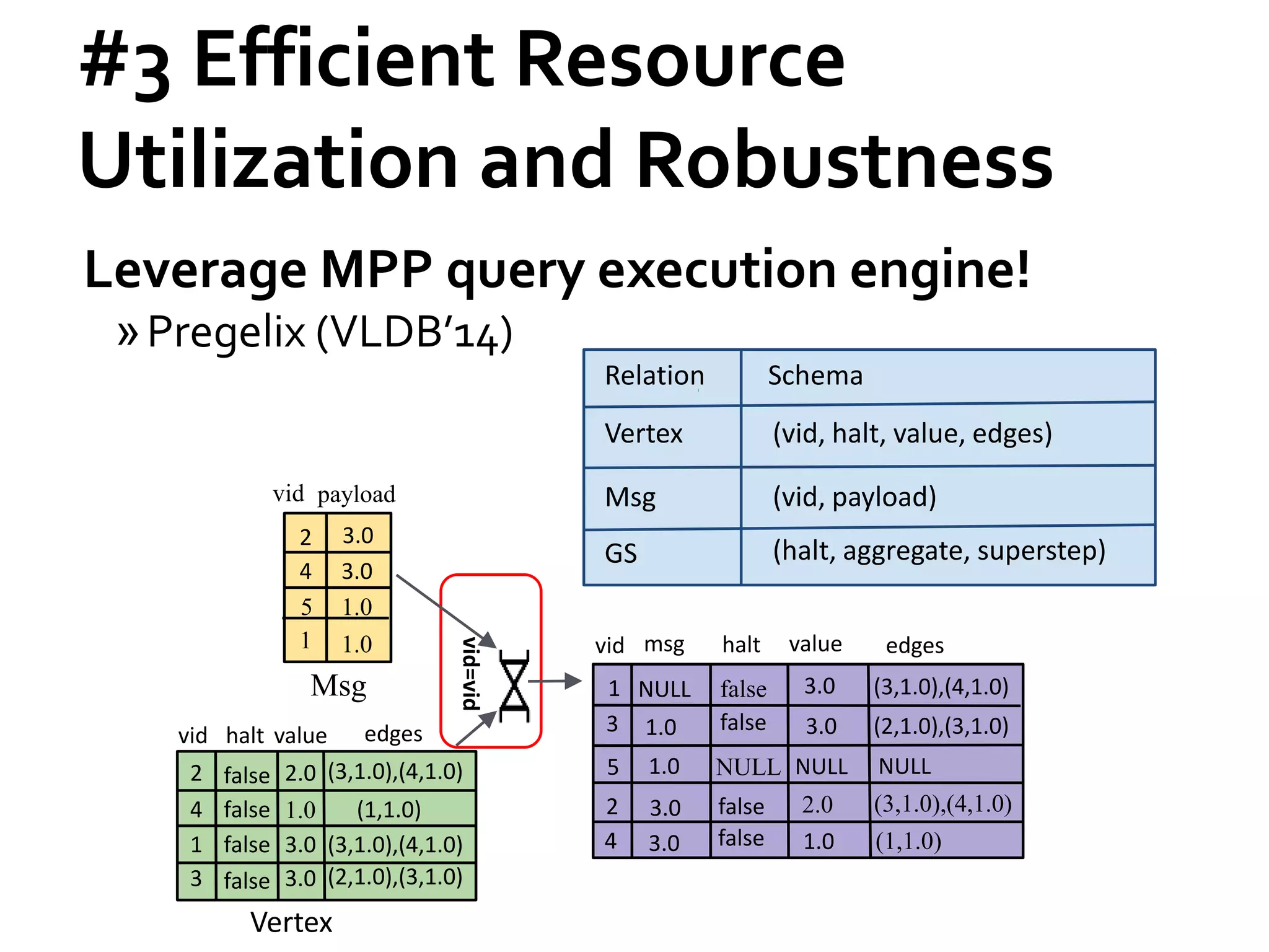
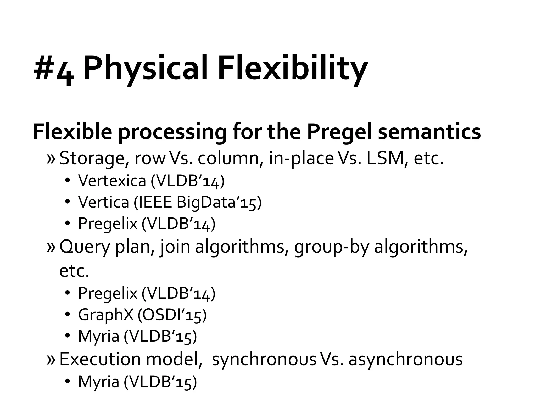
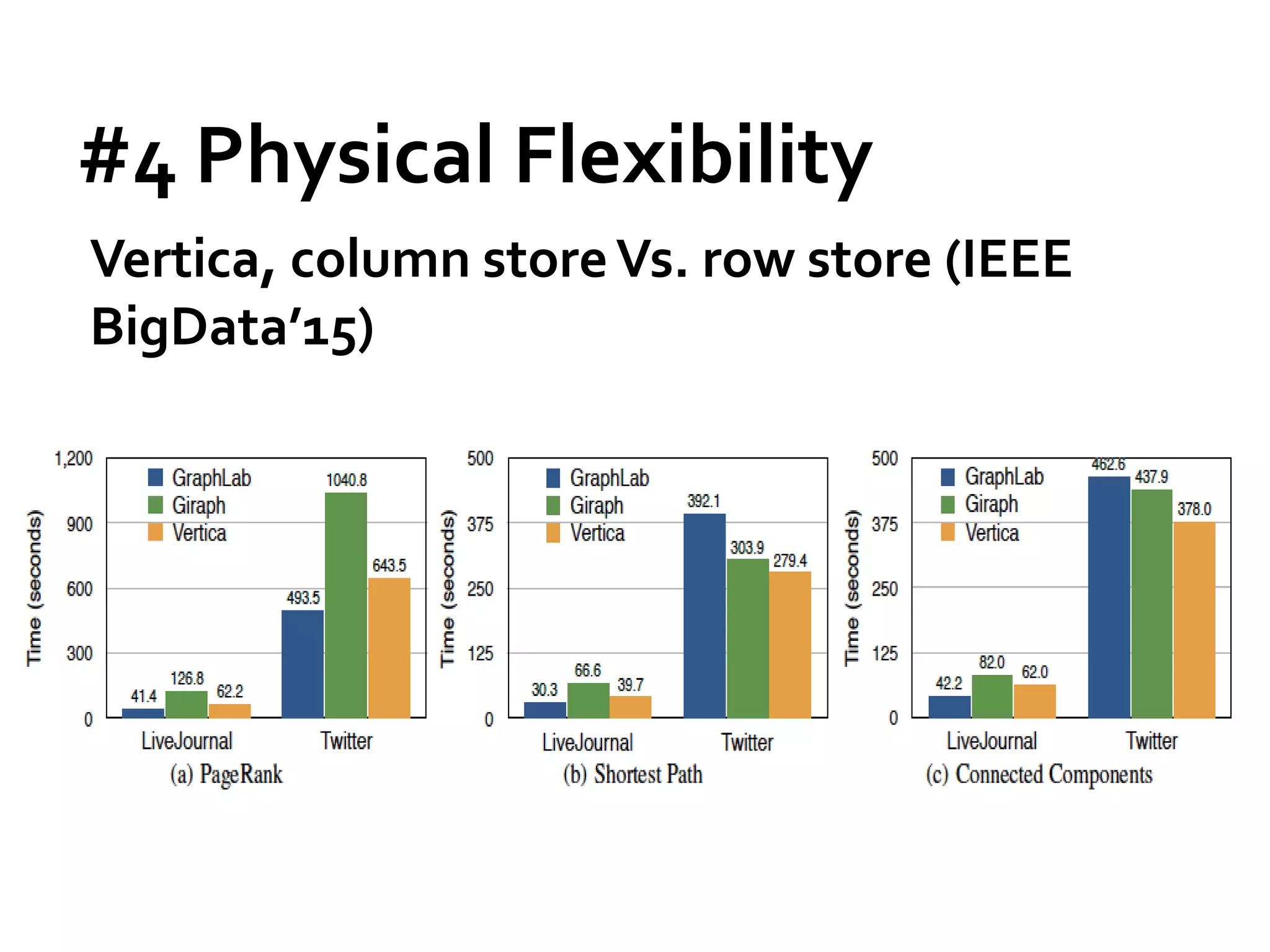
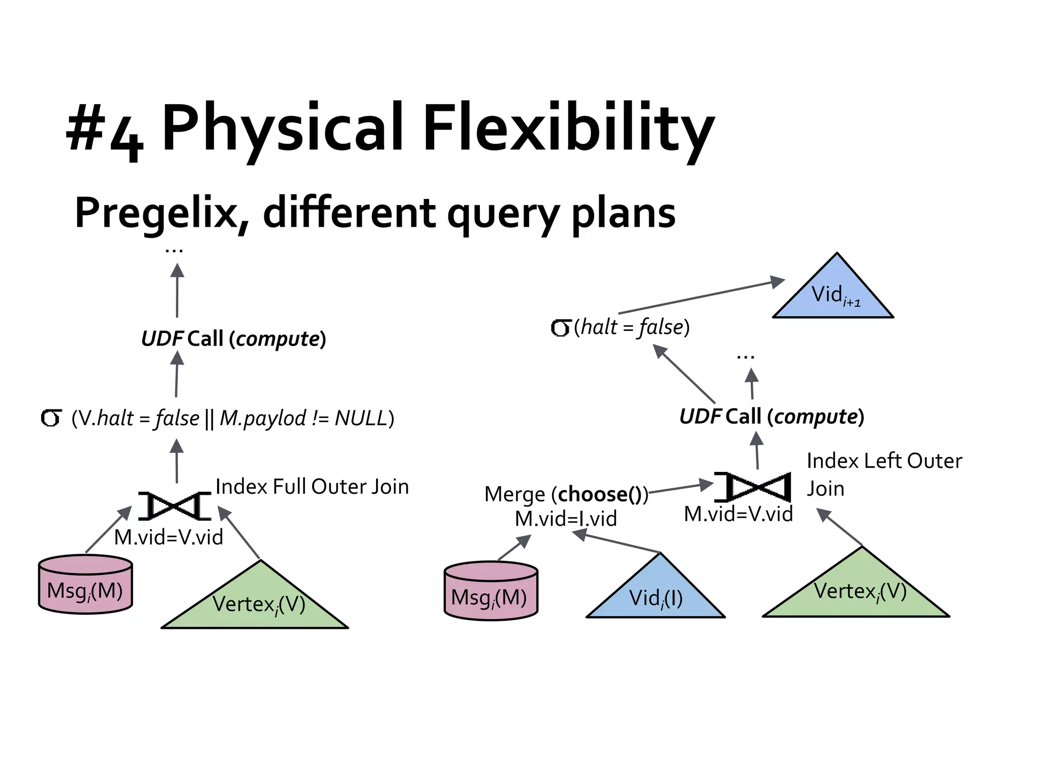
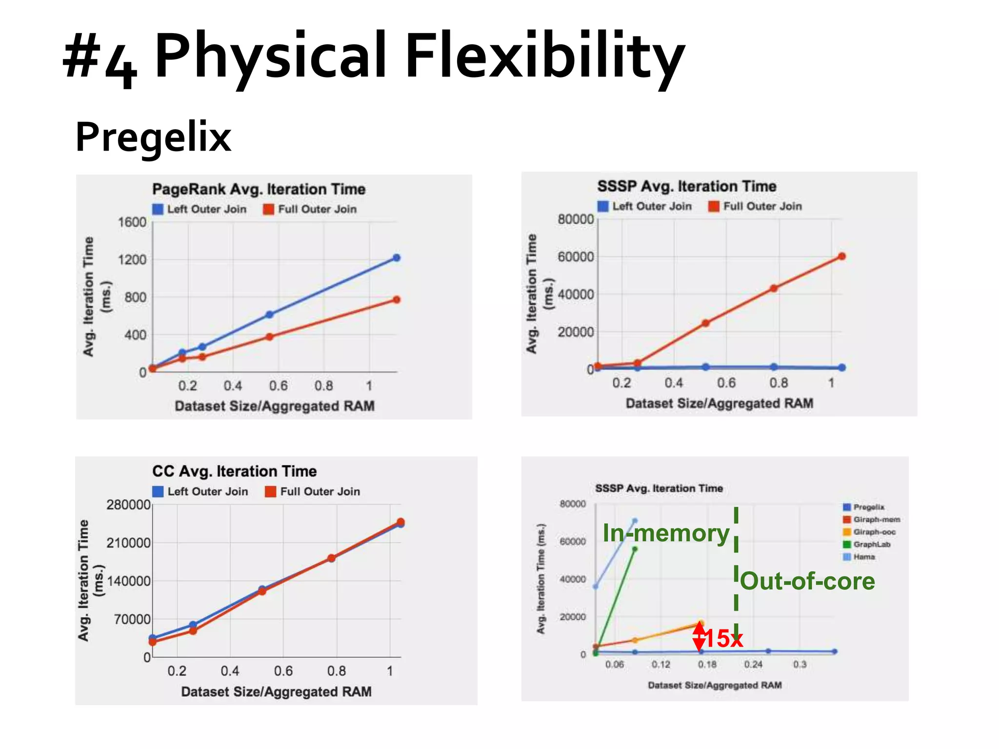
Pregelix [PVLDB’15]
»Transparent out-of-core support
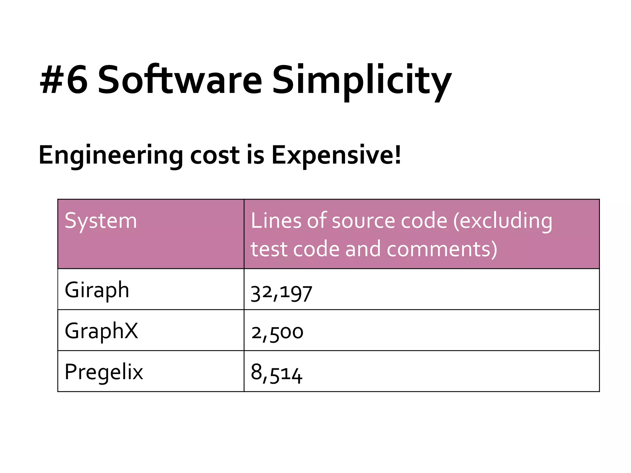
»Physical flexibility (Environment)
»Software simplicity (Implementation)
Hyracks
Dataflow Engine](https://image.slidesharecdn.com/sigmod16tutorial-160706202924/75/Big-Graph-Analytics-Systems-Sigmod16-Tutorial-51-2048.jpg)
![Message Passing Systems
52
Pregelix [PVLDB’15]](https://image.slidesharecdn.com/sigmod16tutorial-160706202924/75/Big-Graph-Analytics-Systems-Sigmod16-Tutorial-52-2048.jpg)
![Message Passing Systems
53
Pregelix [PVLDB’15]](https://image.slidesharecdn.com/sigmod16tutorial-160706202924/75/Big-Graph-Analytics-Systems-Sigmod16-Tutorial-53-2048.jpg)
![Message Passing Systems
59
Chandy-Lamport Snapshot [TOCS’85]
»Uncoordinated checkpointing (e.g., for async exec)
»For message-passing systems
»FIFO channels
u v
5 5
u : 5](https://image.slidesharecdn.com/sigmod16tutorial-160706202924/75/Big-Graph-Analytics-Systems-Sigmod16-Tutorial-59-2048.jpg)
![Message Passing Systems
60
Chandy-Lamport Snapshot [TOCS’85]
»Uncoordinated checkpointing (e.g., for async exec)
»For message-passing systems
»FIFO channels
u v
u : 5
4
4
5](https://image.slidesharecdn.com/sigmod16tutorial-160706202924/75/Big-Graph-Analytics-Systems-Sigmod16-Tutorial-60-2048.jpg)
![Message Passing Systems
61
Chandy-Lamport Snapshot [TOCS’85]
»Uncoordinated checkpointing (e.g., for async exec)
»For message-passing systems
»FIFO channels
u v
u : 5
4 4](https://image.slidesharecdn.com/sigmod16tutorial-160706202924/75/Big-Graph-Analytics-Systems-Sigmod16-Tutorial-61-2048.jpg)
![Message Passing Systems
62
Chandy-Lamport Snapshot [TOCS’85]
»Uncoordinated checkpointing (e.g., for async exec)
»For message-passing systems
»FIFO channels
u v
u : 5 v : 4
4 4](https://image.slidesharecdn.com/sigmod16tutorial-160706202924/75/Big-Graph-Analytics-Systems-Sigmod16-Tutorial-62-2048.jpg)
![Message Passing Systems
63
Chandy-Lamport Snapshot [TOCS’85]
»Solution: bcast checkpoint request right after
checkpointed
u v
5 5
u : 5
REQ
v : 5](https://image.slidesharecdn.com/sigmod16tutorial-160706202924/75/Big-Graph-Analytics-Systems-Sigmod16-Tutorial-63-2048.jpg)
![Message Passing Systems
64
Recovery by Message-Logging [PVLDB’14]
»Each worker logs its msgs to local disks
• Negligible overhead, cost hidden
»Survivor
• No re-computaton during recovery
• Forward logged msgs to replacing workers
»Replacing worker
• Re-compute from latest checkpoint
• Only send msgs to replacing workers](https://image.slidesharecdn.com/sigmod16tutorial-160706202924/75/Big-Graph-Analytics-Systems-Sigmod16-Tutorial-64-2048.jpg)
![Message Passing Systems
65
Recovery by Message-Logging [PVLDB’14]
W1 W2 W3
…
…
…
Superstep
4
W1 W2 W3
5
W2 W3
6
W1 W2 W3
7
Failure occurs
W1
Log msgsLog msgsLog msgs
Log msgsLog msgsLog msgs](https://image.slidesharecdn.com/sigmod16tutorial-160706202924/75/Big-Graph-Analytics-Systems-Sigmod16-Tutorial-65-2048.jpg)
![Message Passing Systems
66
Recovery by Message-Logging [PVLDB’14]
W1 W2 W3
…
…
…
Superstep
4
W1 W2 W3
5
W1 W2 W3
6
W1 W2 W3
7
Standby Machine
Load checkpoint](https://image.slidesharecdn.com/sigmod16tutorial-160706202924/75/Big-Graph-Analytics-Systems-Sigmod16-Tutorial-66-2048.jpg)

![Message Passing Systems
71
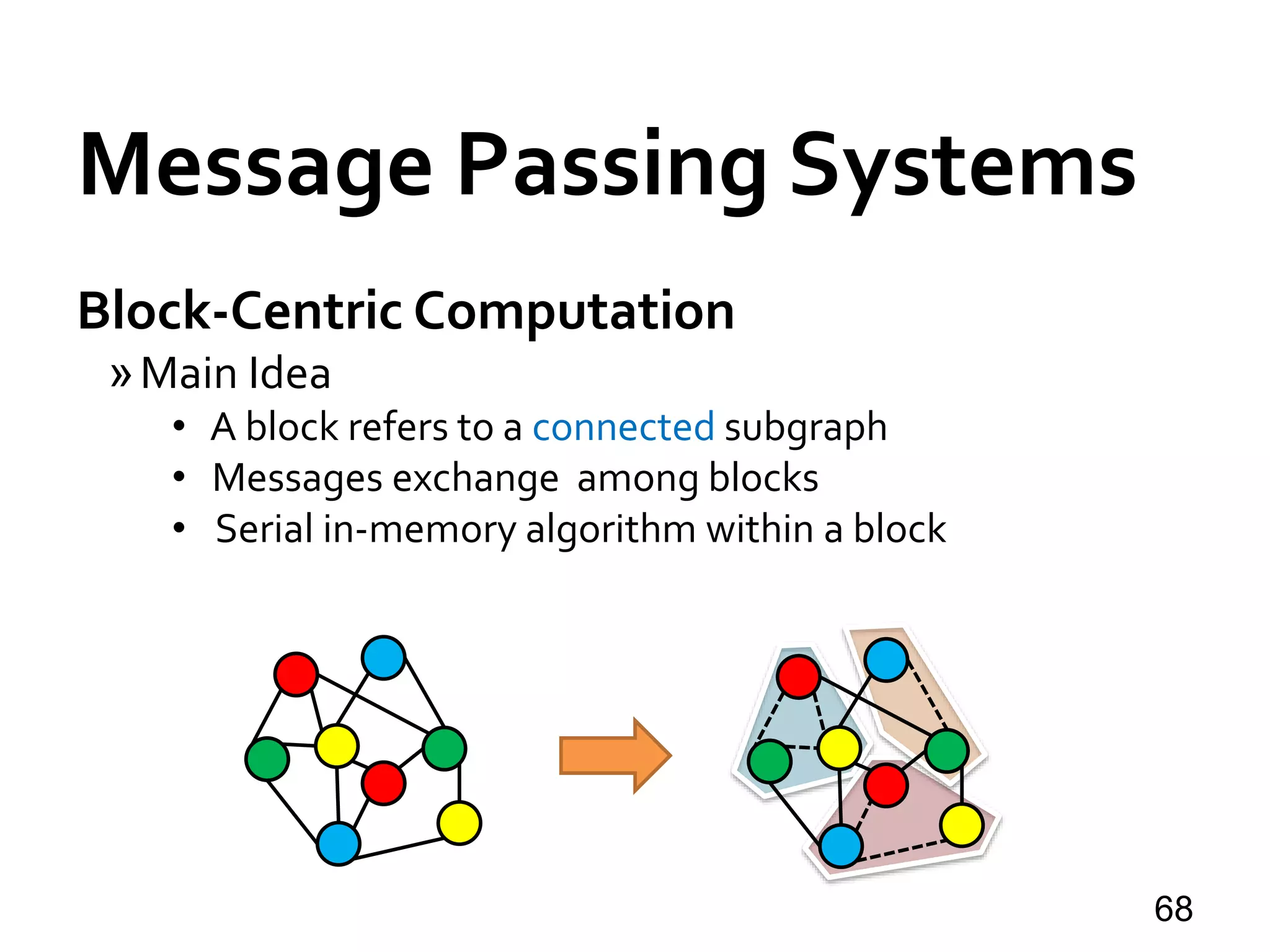
Giraph++ [PVLDB’13]
» Pioneering: think like a graph
» METIS-style vertex partitioning
» Partition.compute(.)
» Boundary vertex values sync-ed at superstep barrier
» Internal vertex values can be updated anytime](https://image.slidesharecdn.com/sigmod16tutorial-160706202924/75/Big-Graph-Analytics-Systems-Sigmod16-Tutorial-71-2048.jpg)
![Message Passing Systems
72
Blogel [PVLDB’14]
» API: vertex.compute(.) + block.compute(.)
»A block can have its own fields
»A block/vertex can send msgs to another block/vertex
»Example: Hash-Min
• Construct block-level graph: to compute an adjacency list
for each block
• Propagate min block ID among blocks](https://image.slidesharecdn.com/sigmod16tutorial-160706202924/75/Big-Graph-Analytics-Systems-Sigmod16-Tutorial-72-2048.jpg)
![Message Passing Systems
73
Blogel [PVLDB’14]
»Performance on Friendster social network with 65.6 M
vertices and 3.6 B edges
1
10
100
1000
2.52
120.24
ComputingTime
Blogel Pregel+
1
100
10,000
19
7,227
MILLION
Total Msg #
Blogel Pregel+
0
10
20
30
5
30
Superstep #
Blogel Pregel+](https://image.slidesharecdn.com/sigmod16tutorial-160706202924/75/Big-Graph-Analytics-Systems-Sigmod16-Tutorial-73-2048.jpg)
![Message Passing Systems
74
Blogel [PVLDB’14]
»Web graph: URL-based partitioning
»Spatial networks: 2D partitioning
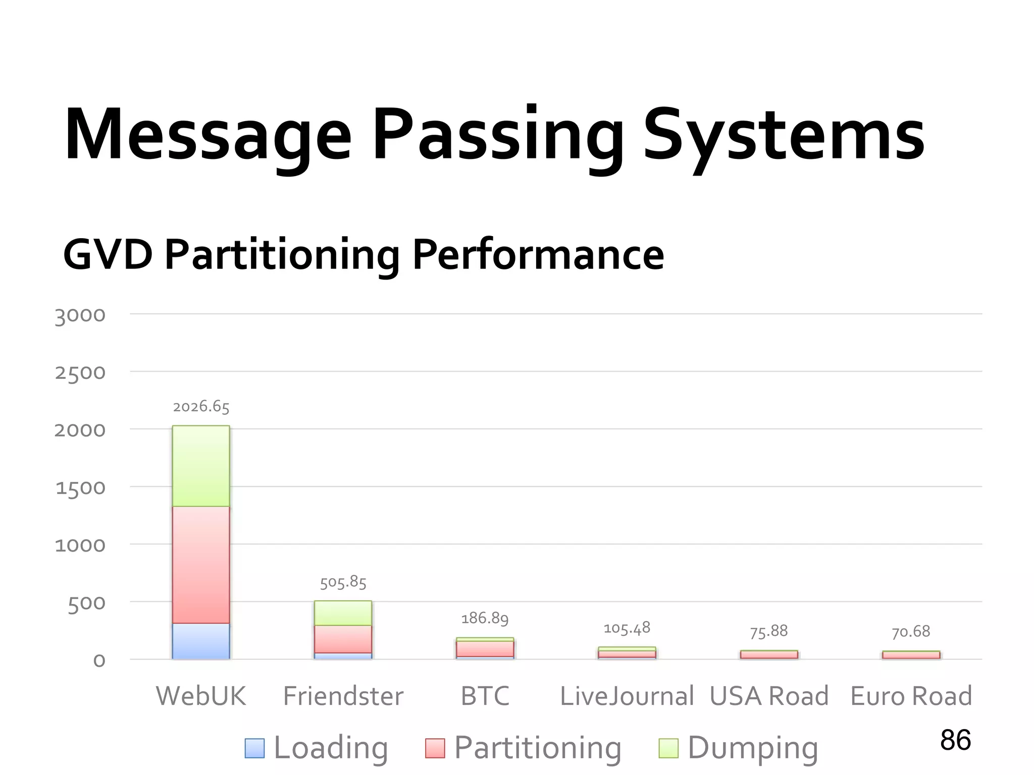
»General graphs: graphVoronoi diagram partitioning](https://image.slidesharecdn.com/sigmod16tutorial-160706202924/75/Big-Graph-Analytics-Systems-Sigmod16-Tutorial-74-2048.jpg)
![Blogel [PVLDB’14]
» GraphVoronoi Diagram (GVD) partitioning
75
Three seeds
v is 2 hops from red seed
v is 3 hops from green seed
v is 5 hops from blue seedv
Message Passing Systems](https://image.slidesharecdn.com/sigmod16tutorial-160706202924/75/Big-Graph-Analytics-Systems-Sigmod16-Tutorial-75-2048.jpg)
![Blogel [PVLDB’14]
»Sample seed vertices with probability p
76
Message Passing Systems](https://image.slidesharecdn.com/sigmod16tutorial-160706202924/75/Big-Graph-Analytics-Systems-Sigmod16-Tutorial-76-2048.jpg)
![Blogel [PVLDB’14]
»Sample seed vertices with probability p
77
Message Passing Systems](https://image.slidesharecdn.com/sigmod16tutorial-160706202924/75/Big-Graph-Analytics-Systems-Sigmod16-Tutorial-77-2048.jpg)
![Blogel [PVLDB’14]
»Sample seed vertices with probability p
»Compute GVD grouping
• Vertex-centric multi-source BFS
78
Message Passing Systems](https://image.slidesharecdn.com/sigmod16tutorial-160706202924/75/Big-Graph-Analytics-Systems-Sigmod16-Tutorial-78-2048.jpg)
![Blogel [PVLDB’14]
79State after Seed Sampling
Message Passing Systems](https://image.slidesharecdn.com/sigmod16tutorial-160706202924/75/Big-Graph-Analytics-Systems-Sigmod16-Tutorial-79-2048.jpg)
![Blogel [PVLDB’14]
80Superstep 1
Message Passing Systems](https://image.slidesharecdn.com/sigmod16tutorial-160706202924/75/Big-Graph-Analytics-Systems-Sigmod16-Tutorial-80-2048.jpg)
![Blogel [PVLDB’14]
81Superstep 2
Message Passing Systems](https://image.slidesharecdn.com/sigmod16tutorial-160706202924/75/Big-Graph-Analytics-Systems-Sigmod16-Tutorial-81-2048.jpg)
![Blogel [PVLDB’14]
82Superstep 3
Message Passing Systems](https://image.slidesharecdn.com/sigmod16tutorial-160706202924/75/Big-Graph-Analytics-Systems-Sigmod16-Tutorial-82-2048.jpg)
![Blogel [PVLDB’14]
»Sample seed vertices with probability p
»Compute GVD grouping
»Postprocessing
83
Message Passing Systems](https://image.slidesharecdn.com/sigmod16tutorial-160706202924/75/Big-Graph-Analytics-Systems-Sigmod16-Tutorial-83-2048.jpg)
![Blogel [PVLDB’14]
»Sample seed vertices with probability p
»Compute GVD grouping
»Postprocessing
• For very large blocks, resample with a larger p and repeat
84
Message Passing Systems](https://image.slidesharecdn.com/sigmod16tutorial-160706202924/75/Big-Graph-Analytics-Systems-Sigmod16-Tutorial-84-2048.jpg)
![Blogel [PVLDB’14]
»Sample seed vertices with probability p
»Compute GVD grouping
»Postprocessing
• For very large blocks, resample with a larger p and repeat
• For tiny components, find them using Hash-Min at last
85
Message Passing Systems](https://image.slidesharecdn.com/sigmod16tutorial-160706202924/75/Big-Graph-Analytics-Systems-Sigmod16-Tutorial-85-2048.jpg)
![Maiter [TPDS’14]
» For algos where vertex values converge asymmetrically
» Delta-based accumulative iterative computation
(DAIC)
88
Message Passing Systems
v1
v2 v3 v4](https://image.slidesharecdn.com/sigmod16tutorial-160706202924/75/Big-Graph-Analytics-Systems-Sigmod16-Tutorial-88-2048.jpg)
![Maiter [TPDS’14]
» For algos where vertex values converge asymmetrically
» Delta-based accumulative iterative computation
(DAIC)
» Strict transformation from Pregel API to DAIC
formulation
»Delta may serve as priority score
»Natural for block-centric frameworks
89
Message Passing Systems](https://image.slidesharecdn.com/sigmod16tutorial-160706202924/75/Big-Graph-Analytics-Systems-Sigmod16-Tutorial-89-2048.jpg)
![Quegel [PVLDB’16]
» On-demand answering of light-workload graph queries
• Only a portion of the whole graph gets accessed
» Option 1: to process queries one job after another
• Network underutilization, too many barriers
• High startup overhead (e.g., graph loading)
91
Message Passing Systems](https://image.slidesharecdn.com/sigmod16tutorial-160706202924/75/Big-Graph-Analytics-Systems-Sigmod16-Tutorial-91-2048.jpg)
![Quegel [PVLDB’16]
» On-demand answering of light-workload graph queries
• Only a portion of the whole graph gets accessed
» Option 2: to process a batch of queries in one job
• Programming complexity
• Straggler problem
92
Message Passing Systems](https://image.slidesharecdn.com/sigmod16tutorial-160706202924/75/Big-Graph-Analytics-Systems-Sigmod16-Tutorial-92-2048.jpg)
![Quegel [PVLDB’16]
»Execution model: superstep-sharing
• Each iteration is called a super-round
• In a super-round, every query proceeds by one superstep
93
Message Passing Systems
Super–Round # 1
q1
2 3 4
1 2 3 4
q3q2 q4
Time
Queries
5 6
q1
q2
q3
q4
7
1 2 3 4
1 2 3 4
1 2 3 4](https://image.slidesharecdn.com/sigmod16tutorial-160706202924/75/Big-Graph-Analytics-Systems-Sigmod16-Tutorial-93-2048.jpg)
![Quegel [PVLDB’16]
»Benefits
• Messages of multiple queries transmitted in one batch
• One synchronization barrier for each super-round
• Better load balancing
94
Message Passing Systems
Worker 1
Worker 2
time sync sync sync
Individual Synchronization Superstep-Sharing](https://image.slidesharecdn.com/sigmod16tutorial-160706202924/75/Big-Graph-Analytics-Systems-Sigmod16-Tutorial-94-2048.jpg)
![Quegel [PVLDB’16]
»API is similar to Pregel
»The system does more:
• Q-data: superstep number, control information, …
• V-data: adjacency list, vertex/edge labels
• VQ-data: vertex state in the evaluation of each query
95
Message Passing Systems](https://image.slidesharecdn.com/sigmod16tutorial-160706202924/75/Big-Graph-Analytics-Systems-Sigmod16-Tutorial-95-2048.jpg)
![Quegel [PVLDB’16]
»Create aVQ-data of v for q, only when q touches v
»Garbage collection of Q-data andVQ-data
»Distributed indexing
96
Message Passing Systems](https://image.slidesharecdn.com/sigmod16tutorial-160706202924/75/Big-Graph-Analytics-Systems-Sigmod16-Tutorial-96-2048.jpg)

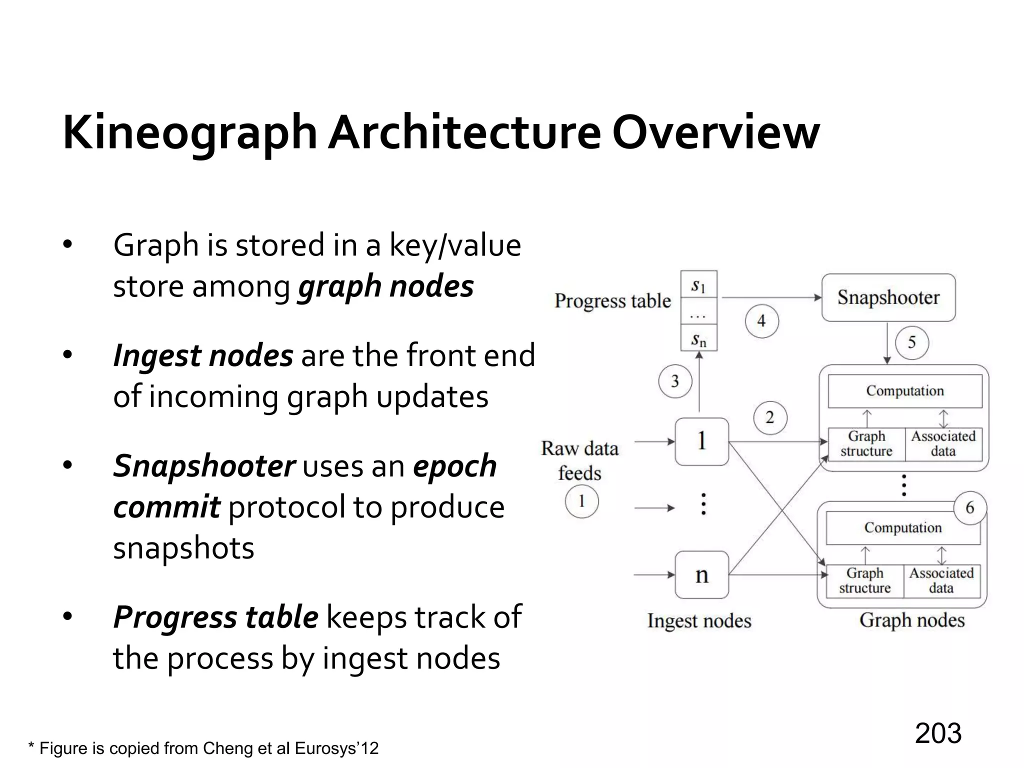
![Shared-Mem Abstraction
Distributed GraphLab [PVLDB’12]
»Scope of vertex v
99
u v w
Du Dv Dw
D(u,v) D(v,w)
…………
…………
All that v can access](https://image.slidesharecdn.com/sigmod16tutorial-160706202924/75/Big-Graph-Analytics-Systems-Sigmod16-Tutorial-99-2048.jpg)
![Shared-Mem Abstraction
Distributed GraphLab [PVLDB’12]
» Async exec mode: for asymmetric convergence
• Scheduler, serializability
» API:v.update()
• Access & update data in v’s scope
• Add neighbors to scheduler
100](https://image.slidesharecdn.com/sigmod16tutorial-160706202924/75/Big-Graph-Analytics-Systems-Sigmod16-Tutorial-100-2048.jpg)
![Shared-Mem Abstraction
Distributed GraphLab [PVLDB’12]
» Vertices partitioned among machines
» For edge (u, v), scopes of u and v overlap
• Du, Dv and D(u, v)
• Replicated if u and v are on different machines
» Ghosts: overlapped boundary data
• Value-sync by a versioning system
» Memory space problem
• x {# of machines}
101](https://image.slidesharecdn.com/sigmod16tutorial-160706202924/75/Big-Graph-Analytics-Systems-Sigmod16-Tutorial-101-2048.jpg)
![Shared-Mem Abstraction
PowerGraph [OSDI’12]
» API: Gather-Apply-Scatter (GAS)
• PageRank: out-degree = 2 for all in-neighbors
102
1
1
1
1
1
1
1
0](https://image.slidesharecdn.com/sigmod16tutorial-160706202924/75/Big-Graph-Analytics-Systems-Sigmod16-Tutorial-102-2048.jpg)
![Shared-Mem Abstraction
PowerGraph [OSDI’12]
» API: Gather-Apply-Scatter (GAS)
• PageRank: out-degree = 2 for all in-neighbors
103
1
1
1
1
1
1
1
1/2
0
1/2
1/2](https://image.slidesharecdn.com/sigmod16tutorial-160706202924/75/Big-Graph-Analytics-Systems-Sigmod16-Tutorial-103-2048.jpg)
![Shared-Mem Abstraction
PowerGraph [OSDI’12]
» API: Gather-Apply-Scatter (GAS)
• PageRank: out-degree = 2 for all in-neighbors
104
1
1
1
1
1
1
1
1.5](https://image.slidesharecdn.com/sigmod16tutorial-160706202924/75/Big-Graph-Analytics-Systems-Sigmod16-Tutorial-104-2048.jpg)
![Shared-Mem Abstraction
PowerGraph [OSDI’12]
» API: Gather-Apply-Scatter (GAS)
• PageRank: out-degree = 2 for all in-neighbors
105
1
1
1
1.5
1
1
1
0
Δ = 0.5 > ϵ](https://image.slidesharecdn.com/sigmod16tutorial-160706202924/75/Big-Graph-Analytics-Systems-Sigmod16-Tutorial-105-2048.jpg)
![Shared-Mem Abstraction
PowerGraph [OSDI’12]
» API: Gather-Apply-Scatter (GAS)
• PageRank: out-degree = 2 for all in-neighbors
106
1
1
1
1.5
1
1
1
0
activated
activated
activated](https://image.slidesharecdn.com/sigmod16tutorial-160706202924/75/Big-Graph-Analytics-Systems-Sigmod16-Tutorial-106-2048.jpg)
![Shared-Mem Abstraction
PowerGraph [OSDI’12]
»Edge Partitioning
»Goals:
• Loading balancing
• Minimize vertex replicas
– Cost of value sync
– Cost of memory space
107](https://image.slidesharecdn.com/sigmod16tutorial-160706202924/75/Big-Graph-Analytics-Systems-Sigmod16-Tutorial-107-2048.jpg)
![Shared-Mem Abstraction
PowerGraph [OSDI’12]
»Greedy Edge Placement
108
u v
W1 W2 W3 W4 W5 W6
Workload 100 101 102 103 104 105](https://image.slidesharecdn.com/sigmod16tutorial-160706202924/75/Big-Graph-Analytics-Systems-Sigmod16-Tutorial-108-2048.jpg)
![Shared-Mem Abstraction
PowerGraph [OSDI’12]
»Greedy Edge Placement
109
u v
W1 W2 W3 W4 W5 W6
Workload 100 101 102 103 104 105](https://image.slidesharecdn.com/sigmod16tutorial-160706202924/75/Big-Graph-Analytics-Systems-Sigmod16-Tutorial-109-2048.jpg)
![Shared-Mem Abstraction
PowerGraph [OSDI’12]
»Greedy Edge Placement
110
u v
W1 W2 W3 W4 W5 W6
Workload 100 101 102 103 104 105
∅ ∅](https://image.slidesharecdn.com/sigmod16tutorial-160706202924/75/Big-Graph-Analytics-Systems-Sigmod16-Tutorial-110-2048.jpg)
![Shared-Mem Abstraction
Shared-Mem + Single-Machine
»Out-of-core execution, disk/SSD-based
• GraphChi [OSDI’12]
• X-Stream [SOSP’13]
• VENUS [ICDE’14]
• …
»Vertices are numbered 1, …, n; cut into P intervals
112
interval(2) interval(P)
1 nv1 v2
interval(1)](https://image.slidesharecdn.com/sigmod16tutorial-160706202924/75/Big-Graph-Analytics-Systems-Sigmod16-Tutorial-112-2048.jpg)
![Shared-Mem Abstraction
GraphChi [OSDI’12]
»Programming Model
• Edge scope of v
113
u v w
Du Dv Dw
D(u,v) D(v,w)
…………
…………](https://image.slidesharecdn.com/sigmod16tutorial-160706202924/75/Big-Graph-Analytics-Systems-Sigmod16-Tutorial-113-2048.jpg)
![Shared-Mem Abstraction
GraphChi [OSDI’12]
»Programming Model
• Scatter & gather values along adjacent edges
114
u v w
Dv
D(u,v) D(v,w)
…………
…………](https://image.slidesharecdn.com/sigmod16tutorial-160706202924/75/Big-Graph-Analytics-Systems-Sigmod16-Tutorial-114-2048.jpg)
![Shared-Mem Abstraction
GraphChi [OSDI’12]
»Load vertices of each interval, along with adjacent
edges for in-mem processing
»Write updated vertex/edge values back to disk
»Challenges
• Sequential IO
• Consistency: store each edge value only once on disk
115
interval(2) interval(P)
1 nv1 v2
interval(1)](https://image.slidesharecdn.com/sigmod16tutorial-160706202924/75/Big-Graph-Analytics-Systems-Sigmod16-Tutorial-115-2048.jpg)
![Shared-Mem Abstraction
GraphChi [OSDI’12]
»Disk shards: shard(i)
• Vertices in interval(i)
• Their incoming edges, sorted by source_ID
116
interval(2) interval(P)
1 nv1 v2
interval(1)
shard(P)shard(2)shard(1)](https://image.slidesharecdn.com/sigmod16tutorial-160706202924/75/Big-Graph-Analytics-Systems-Sigmod16-Tutorial-116-2048.jpg)
![Shared-Mem Abstraction
GraphChi [OSDI’12]
»Parallel SlidingWindows (PSW)
117
Shard 1
in-edgessortedby
src_id
Vertices
1..100
Vertices
101..200
Vertices
201..300
Vertices
301..400
Shard 2 Shard 3 Shard 4Shard 1](https://image.slidesharecdn.com/sigmod16tutorial-160706202924/75/Big-Graph-Analytics-Systems-Sigmod16-Tutorial-117-2048.jpg)
![Shared-Mem Abstraction
GraphChi [OSDI’12]
»Parallel SlidingWindows (PSW)
118
Shard 1
in-edgessortedby
src_id
Vertices
1..100
Vertices
101..200
Vertices
201..300
Vertices
301..400
Shard 2 Shard 3 Shard 4Shard 1
100
100
100
1 1 1 1
Out-Edges
Vertices & In-Edges
100](https://image.slidesharecdn.com/sigmod16tutorial-160706202924/75/Big-Graph-Analytics-Systems-Sigmod16-Tutorial-118-2048.jpg)
![Shared-Mem Abstraction
GraphChi [OSDI’12]
»Parallel SlidingWindows (PSW)
119
Shard 1
in-edgessortedby
src_id
Vertices
1..100
Vertices
101..200
Vertices
201..300
Vertices
301..400
Shard 2 Shard 3 Shard 4Shard 1
1 1 1 1
100
100
100
200
Vertices & In-Edges
200
200
Out-Edges
100
200](https://image.slidesharecdn.com/sigmod16tutorial-160706202924/75/Big-Graph-Analytics-Systems-Sigmod16-Tutorial-119-2048.jpg)
![Shared-Mem Abstraction
GraphChi [OSDI’12]
»Each vertex & edge value is read & written for at least
once in an iteration
120](https://image.slidesharecdn.com/sigmod16tutorial-160706202924/75/Big-Graph-Analytics-Systems-Sigmod16-Tutorial-120-2048.jpg)
![Shared-Mem Abstraction
X-Stream [SOSP’13]
»Edge-scope GAS programming model
»Streams a completely unordered list of edges
121](https://image.slidesharecdn.com/sigmod16tutorial-160706202924/75/Big-Graph-Analytics-Systems-Sigmod16-Tutorial-121-2048.jpg)
![Shared-Mem Abstraction
X-Stream [SOSP’13]
»Simple case: all vertex states are memory-resident
»Pass 1: edge-centric scattering
• (u, v): value(u) => <v, value(u, v)>
»Pass 2: edge-centric gathering
• <v, value(u, v)> => value(v)
122
update
aggregate](https://image.slidesharecdn.com/sigmod16tutorial-160706202924/75/Big-Graph-Analytics-Systems-Sigmod16-Tutorial-122-2048.jpg)
![Shared-Mem Abstraction
X-Stream [SOSP’13]
»Out-of-Core Engine
• P vertex partitions with vertex states only
• P edge partitions, partitioned by source vertices
• Each pass loads a vertex partition, streams corresponding
edge partition (or update partition)
123
interval(2) interval(P)
1 nv1 v2
interval(1)
Fit into memory
Larger than in GraphChi
Streamed on disk
P update files generated by Pass 1 scattering](https://image.slidesharecdn.com/sigmod16tutorial-160706202924/75/Big-Graph-Analytics-Systems-Sigmod16-Tutorial-123-2048.jpg)
![Shared-Mem Abstraction
X-Stream [SOSP’13]
»Out-of-Core Engine
• Pass 1: edge-centric scattering
– (u, v): value(u) => [v, value(u, v)]
• Pass 2: edge-centric scattering
– [v, value(u, v)] => value(v)
124
interval(2) interval(P)
1 nv1 v2
interval(1)
Append to update file
for partition of v
Streamed from update file
for the corresponding vertex partition](https://image.slidesharecdn.com/sigmod16tutorial-160706202924/75/Big-Graph-Analytics-Systems-Sigmod16-Tutorial-124-2048.jpg)
![Shared-Mem Abstraction
X-Stream [SOSP’13]
»Scale out: Chaos [SOSP’15]
• Requires 40 GigE
• Slow with GigE
»Weakness: sparse computation
125](https://image.slidesharecdn.com/sigmod16tutorial-160706202924/75/Big-Graph-Analytics-Systems-Sigmod16-Tutorial-125-2048.jpg)
![Shared-Mem Abstraction
VENUS [ICDE’14]
»Programming model
• Value scope of v
126
u v w
Du Dv Dw
D(u,v) D(v,w)
…………
…………](https://image.slidesharecdn.com/sigmod16tutorial-160706202924/75/Big-Graph-Analytics-Systems-Sigmod16-Tutorial-126-2048.jpg)
![Shared-Mem Abstraction
VENUS [ICDE’14]
»Assume static topology
• Separate read-only edge data and mutable vertex states
»g-shard(i): incoming edge lists of vertices in interval(i)
»v-shard(i): srcs & dsts of edges in g-shard(i)
»All g-shards are concatenated for streaming
127
interval(2) interval(P)
1 nv1 v2
interval(1)
Sources may not be in interval(i)
Vertices in a v-shard are ordered by ID](https://image.slidesharecdn.com/sigmod16tutorial-160706202924/75/Big-Graph-Analytics-Systems-Sigmod16-Tutorial-127-2048.jpg)
![Dsts of interval(i) may be srcs of other intervals
Shared-Mem Abstraction
VENUS [ICDE’14]
»To process interval(i)
• Load v-shard(i)
• Stream g-shard(i), update in-memory v-shard(i)
• Update every other v-shard by a sequential write
128
interval(2) interval(P)
1 nv1 v2
interval(1)
Dst vertices are in interval(i)](https://image.slidesharecdn.com/sigmod16tutorial-160706202924/75/Big-Graph-Analytics-Systems-Sigmod16-Tutorial-128-2048.jpg)
![Shared-Mem Abstraction
VENUS [ICDE’14]
» Avoid writing O(|E|) edge values to disk
» O(|E|) edge values are read once
» O(|V|) may be read/written for multiple times
129
interval(2) interval(P)
1 nv1 v2
interval(1)](https://image.slidesharecdn.com/sigmod16tutorial-160706202924/75/Big-Graph-Analytics-Systems-Sigmod16-Tutorial-129-2048.jpg)

![Single-Machine Systems
TurboGraph [KDD’13]
»Vertices ordered by ID, stored in pages
134](https://image.slidesharecdn.com/sigmod16tutorial-160706202924/75/Big-Graph-Analytics-Systems-Sigmod16-Tutorial-134-2048.jpg)
![Single-Machine Systems
TurboGraph [KDD’13]
135](https://image.slidesharecdn.com/sigmod16tutorial-160706202924/75/Big-Graph-Analytics-Systems-Sigmod16-Tutorial-135-2048.jpg)
![Single-Machine Systems
TurboGraph [KDD’13]
136
Read order for positions in a page](https://image.slidesharecdn.com/sigmod16tutorial-160706202924/75/Big-Graph-Analytics-Systems-Sigmod16-Tutorial-136-2048.jpg)
![Single-Machine Systems
TurboGraph [KDD’13]
137
Record for v6: in Page p3, Position 1](https://image.slidesharecdn.com/sigmod16tutorial-160706202924/75/Big-Graph-Analytics-Systems-Sigmod16-Tutorial-137-2048.jpg)
![Single-Machine Systems
TurboGraph [KDD’13]
138
In-mem page table: vertex ID -> location on SSD
1-hop neighborhood: outperform GraphChi by 104](https://image.slidesharecdn.com/sigmod16tutorial-160706202924/75/Big-Graph-Analytics-Systems-Sigmod16-Tutorial-138-2048.jpg)
![Single-Machine Systems
TurboGraph [KDD’13]
139
Special treatment for adj-list larger than a page](https://image.slidesharecdn.com/sigmod16tutorial-160706202924/75/Big-Graph-Analytics-Systems-Sigmod16-Tutorial-139-2048.jpg)
![Single-Machine Systems
TurboGraph [KDD’13]
»Pin-and-slide execution model
»Concurrently process vertices of pinned pages
»Do not wait for completion of IO requests
»Page unpinned as soon as processed
140](https://image.slidesharecdn.com/sigmod16tutorial-160706202924/75/Big-Graph-Analytics-Systems-Sigmod16-Tutorial-140-2048.jpg)
![Single-Machine Systems
FlashGraph [FAST’15]
»Semi-external memory
• Edge lists on SSDs
»On top of SAFS, an SSD file system
• High-throughput async I/Os over SSD array
• Edge lists stored in one (logical) file on SSD
141](https://image.slidesharecdn.com/sigmod16tutorial-160706202924/75/Big-Graph-Analytics-Systems-Sigmod16-Tutorial-141-2048.jpg)
![Single-Machine Systems
FlashGraph [FAST’15]
»Only access requested edge lists
»Merge same-page / adjacent-page requests into one
sequential access
»Vertex-centricAPI
»Message passing among threads
142](https://image.slidesharecdn.com/sigmod16tutorial-160706202924/75/Big-Graph-Analytics-Systems-Sigmod16-Tutorial-142-2048.jpg)

![Single-Machine Systems
Green-Marl [ASPLOS’12]
»Domain-specific language (DSL)
• High-level language constructs
• Expose data-level parallelism
»DSL → C++ program
»Initially single-machine, now supported by GPS
145](https://image.slidesharecdn.com/sigmod16tutorial-160706202924/75/Big-Graph-Analytics-Systems-Sigmod16-Tutorial-145-2048.jpg)
![Single-Machine Systems
Green-Marl [ASPLOS’12]
»Parallel For
»Parallel BFS
»Reductions (e.g., SUM, MIN, AND)
»Deferred assignment (<=)
• Effective only at the end of the binding iteration
146](https://image.slidesharecdn.com/sigmod16tutorial-160706202924/75/Big-Graph-Analytics-Systems-Sigmod16-Tutorial-146-2048.jpg)
![Single-Machine Systems
Ligra [PPoPP’13]
»VertexSet-centric API: edgeMap, vertexMap
»Example: BFS
• Ui+1←edgeMap(Ui, F, C)
147
u
v
Ui
Vertices for next iteration](https://image.slidesharecdn.com/sigmod16tutorial-160706202924/75/Big-Graph-Analytics-Systems-Sigmod16-Tutorial-147-2048.jpg)
![Single-Machine Systems
Ligra [PPoPP’13]
»VertexSet-centric API: edgeMap, vertexMap
»Example: BFS
• Ui+1←edgeMap(Ui, F, C)
148
u
v
Ui
C(v) = parent[v] is NULL?
Yes](https://image.slidesharecdn.com/sigmod16tutorial-160706202924/75/Big-Graph-Analytics-Systems-Sigmod16-Tutorial-148-2048.jpg)
![Single-Machine Systems
Ligra [PPoPP’13]
»VertexSet-centric API: edgeMap, vertexMap
»Example: BFS
• Ui+1←edgeMap(Ui, F, C)
149
u
v
Ui
F(u, v):
parent[v] ← u
v added to Ui+1](https://image.slidesharecdn.com/sigmod16tutorial-160706202924/75/Big-Graph-Analytics-Systems-Sigmod16-Tutorial-149-2048.jpg)
![Single-Machine Systems
Ligra [PPoPP’13]
»Mode switch based on vertex sparseness |Ui|
• When | Ui | is large
150
u
v
Ui
w
C(w) called 3 times](https://image.slidesharecdn.com/sigmod16tutorial-160706202924/75/Big-Graph-Analytics-Systems-Sigmod16-Tutorial-150-2048.jpg)
![Single-Machine Systems
Ligra [PPoPP’13]
»Mode switch based on vertex sparseness |Ui|
• When | Ui | is large
151
u
v
Ui
w
if C(v) is true
Call F(u, v) for every in-neighbor in U
Early pruning: just the first one for BFS](https://image.slidesharecdn.com/sigmod16tutorial-160706202924/75/Big-Graph-Analytics-Systems-Sigmod16-Tutorial-151-2048.jpg)
![Single-Machine Systems
GRACE [PVLDB’13]
»Vertex-centricAPI, block-centric execution
• Inner-block computation: vertex-centric computation with
an inner-block scheduler
»Reduce data access to computation ratio
• Many vertex-centric algos are computationally-light
• CPU cache locality: every block fits in cache
152](https://image.slidesharecdn.com/sigmod16tutorial-160706202924/75/Big-Graph-Analytics-Systems-Sigmod16-Tutorial-152-2048.jpg)
![Single-Machine Systems
Galois [SOSP’13]
»Amorphous data-parallelism (ADP)
• Speculative execution: fully use extra CPU resources
153
v’s neighborhoodu’s neighborhood
u vw](https://image.slidesharecdn.com/sigmod16tutorial-160706202924/75/Big-Graph-Analytics-Systems-Sigmod16-Tutorial-153-2048.jpg)
![Single-Machine Systems
Galois [SOSP’13]
»Amorphous data-parallelism (ADP)
• Speculative execution: fully use extra CPU resources
154
v’s neighborhoodu’s neighborhood
u vw
Rollback](https://image.slidesharecdn.com/sigmod16tutorial-160706202924/75/Big-Graph-Analytics-Systems-Sigmod16-Tutorial-154-2048.jpg)
![Single-Machine Systems
Galois [SOSP’13]
»Amorphous data-parallelism (ADP)
• Speculative execution: fully use extra CPU resources
»Machine-topology-aware scheduler
• Try to fetch tasks local to the current core first
155](https://image.slidesharecdn.com/sigmod16tutorial-160706202924/75/Big-Graph-Analytics-Systems-Sigmod16-Tutorial-155-2048.jpg)
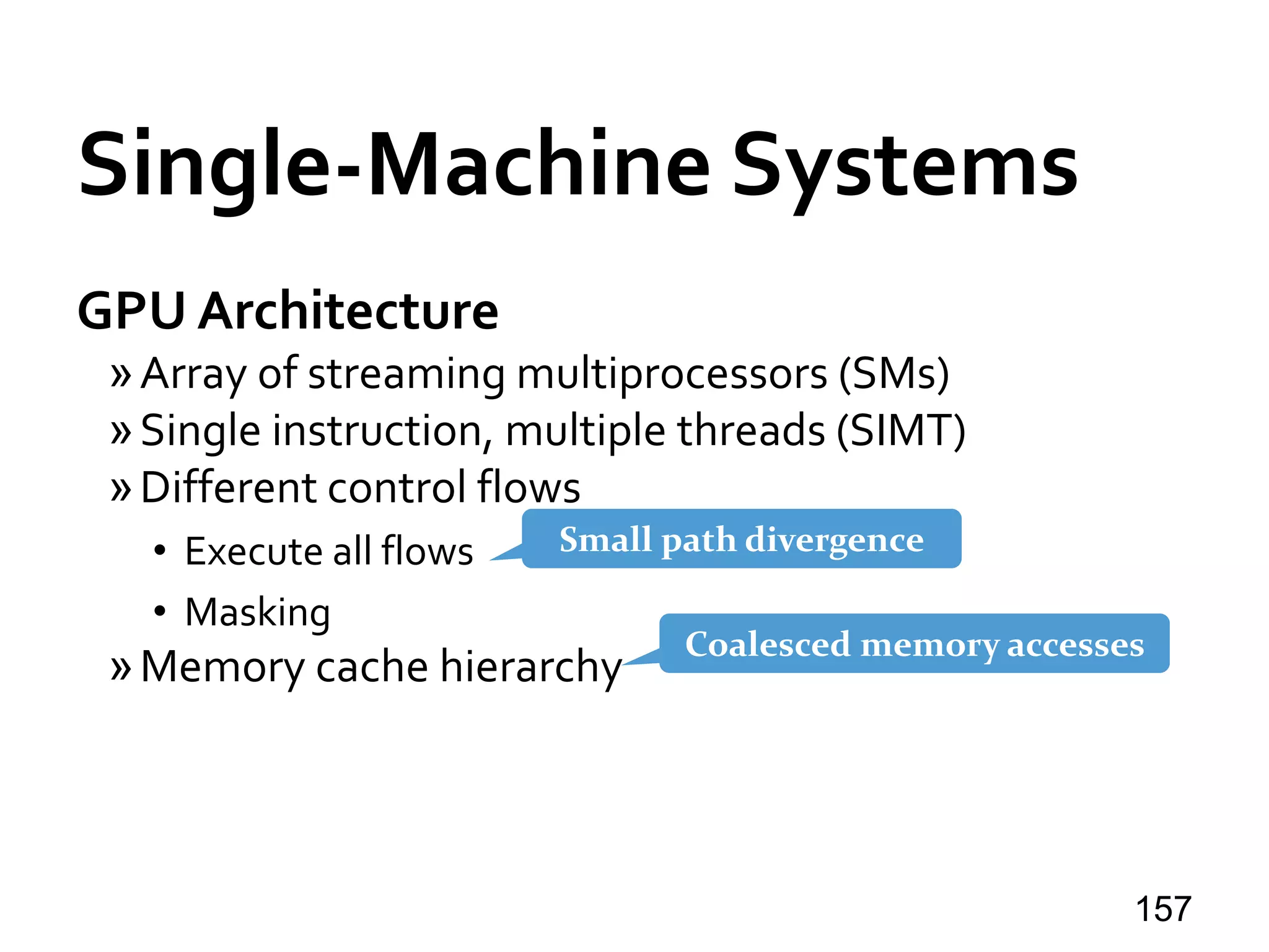
![Single-Machine Systems
Medusa [TPDS’14]
»BPS model of Pregel
»Fine-grained API: Edge-Message-Vertex (EMV)
• Large parallelism, small path divergence
»Pre-allocates an array for buffering messages
• Coalesced memory accesses: incoming msgs for each vertex
is consecutive
• Write positions of msgs do not conflict
159](https://image.slidesharecdn.com/sigmod16tutorial-160706202924/75/Big-Graph-Analytics-Systems-Sigmod16-Tutorial-159-2048.jpg)
![Single-Machine Systems
CuSha [HPDC’14]
»Apply the shard organization of GraphChi
»Each shard processed by one CTA
»Window concatenation
160
Window write-back: imbalanced workload
Shard 1
n-edgessortedbysrc_id
Vertices
1..100
Vertices
101..200
Vertices
201..300
Vertices
301..400
Shard 2 Shard 3 Shard 4Shard 1
1 1 1 1
100
100
100
200 200
200
100
200](https://image.slidesharecdn.com/sigmod16tutorial-160706202924/75/Big-Graph-Analytics-Systems-Sigmod16-Tutorial-160-2048.jpg)
![Single-Machine Systems
CuSha [HPDC’14]
»Apply the shard organization of GraphChi
»Each shard processed by one CTA
»Window concatenation
161
Threads in a CTA may
cross window boundaries
Pointers to actual locations
in shards
Window write-back: imbalanced workload](https://image.slidesharecdn.com/sigmod16tutorial-160706202924/75/Big-Graph-Analytics-Systems-Sigmod16-Tutorial-161-2048.jpg)

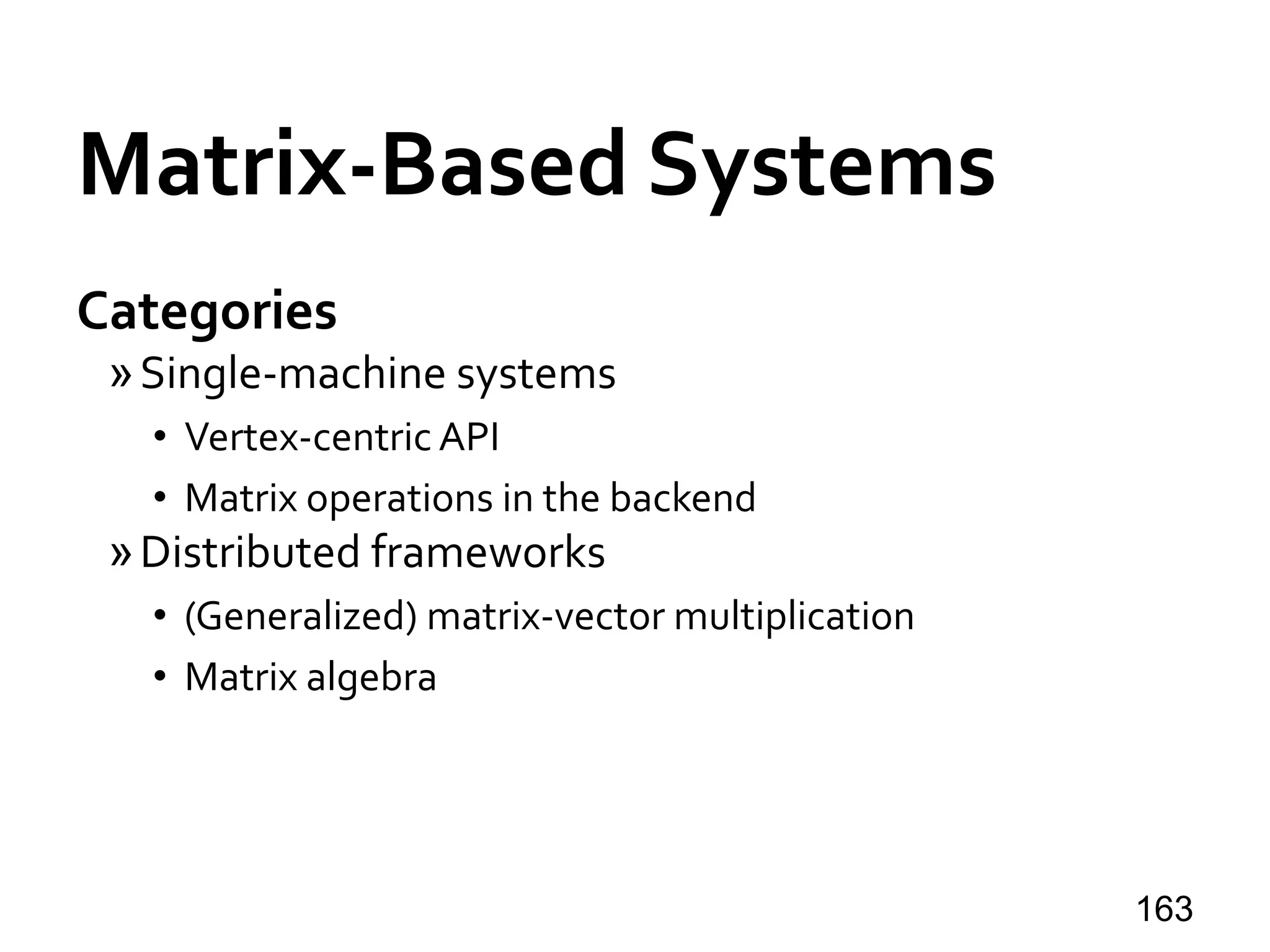
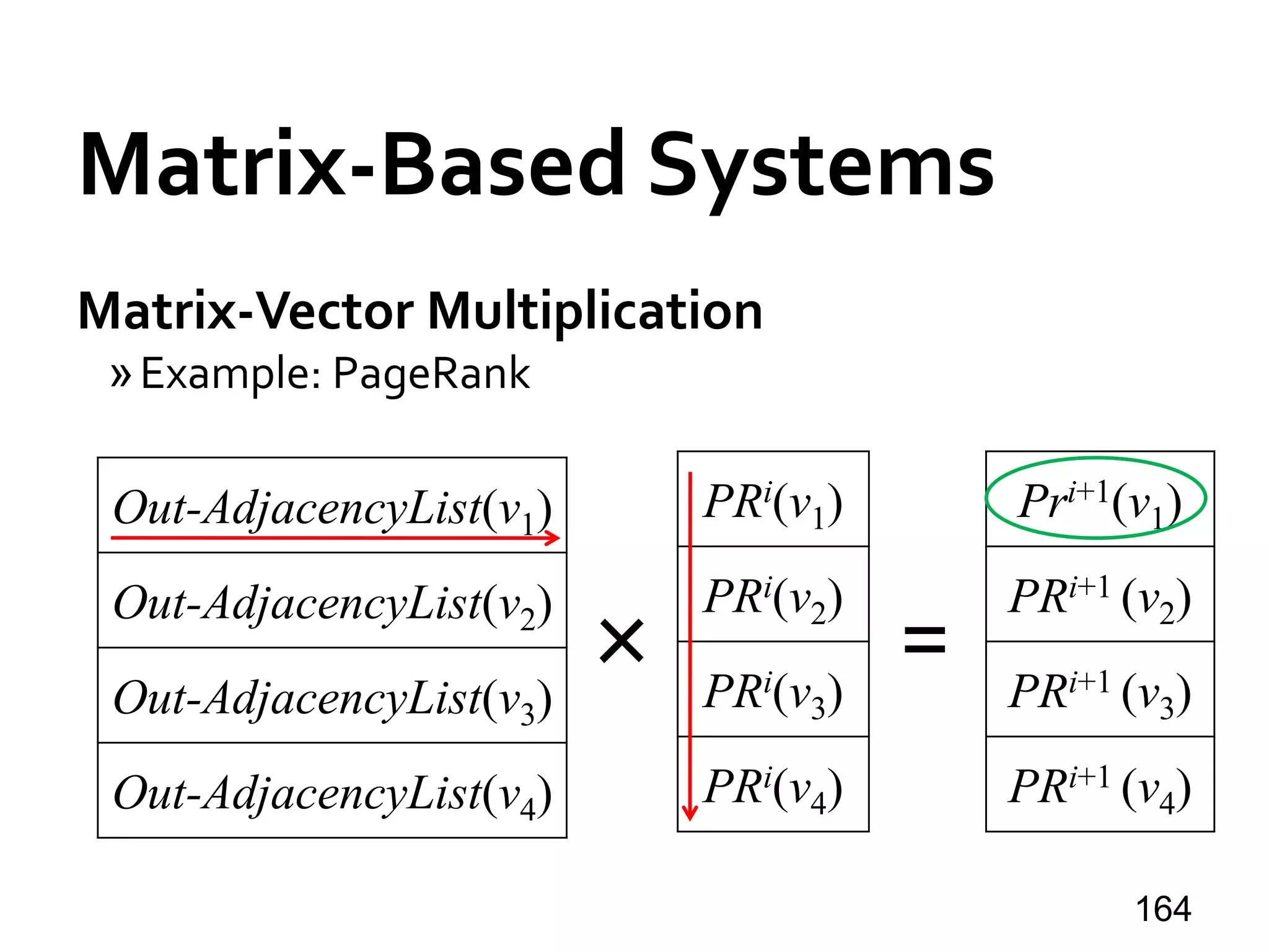
![Matrix-Based Systems
GraphTwist [PVLDB’15]
»Multi-level graph partitioning
• Right granularity for in-memory processing
• Balance workloads among computing threads
1671 n
src
dst
1
n
u
v
w(u, v)
edge-weight](https://image.slidesharecdn.com/sigmod16tutorial-160706202924/75/Big-Graph-Analytics-Systems-Sigmod16-Tutorial-167-2048.jpg)
![Matrix-Based Systems
GraphTwist [PVLDB’15]
»Multi-level graph partitioning
• Right granularity for in-memory processing
• Balance workloads among computing threads
1681 n
src
dst
1
n
edge-weight
slice](https://image.slidesharecdn.com/sigmod16tutorial-160706202924/75/Big-Graph-Analytics-Systems-Sigmod16-Tutorial-168-2048.jpg)
![Matrix-Based Systems
GraphTwist [PVLDB’15]
»Multi-level graph partitioning
• Right granularity for in-memory processing
• Balance workloads among computing threads
1691 n
src
dst
1
n
edge-weight
stripe](https://image.slidesharecdn.com/sigmod16tutorial-160706202924/75/Big-Graph-Analytics-Systems-Sigmod16-Tutorial-169-2048.jpg)
![Matrix-Based Systems
GraphTwist [PVLDB’15]
»Multi-level graph partitioning
• Right granularity for in-memory processing
• Balance workloads among computing threads
1701 n
src
dst
1
n
edge-weight
dice](https://image.slidesharecdn.com/sigmod16tutorial-160706202924/75/Big-Graph-Analytics-Systems-Sigmod16-Tutorial-170-2048.jpg)
![Matrix-Based Systems
GraphTwist [PVLDB’15]
»Multi-level graph partitioning
• Right granularity for in-memory processing
• Balance workloads among computing threads
1711 n
src
dst
1
n
edge-weight
u
vertex cut](https://image.slidesharecdn.com/sigmod16tutorial-160706202924/75/Big-Graph-Analytics-Systems-Sigmod16-Tutorial-171-2048.jpg)
![Matrix-Based Systems
GraphTwist [PVLDB’15]
»Multi-level graph partitioning
• Right granularity for in-memory processing
• Balance workloads among computing threads
»Fast Randomized Approximation
• Prune statistically insignificant vertices/edges
• E.g., PageRank computation only using high-weight edges
• Unbiased estimator: sampling slices/cuts according to
Frobenius norm
172](https://image.slidesharecdn.com/sigmod16tutorial-160706202924/75/Big-Graph-Analytics-Systems-Sigmod16-Tutorial-172-2048.jpg)
![Matrix-Based Systems
GridGraph [ATC’15]
»Grid representation for reducing IO
173](https://image.slidesharecdn.com/sigmod16tutorial-160706202924/75/Big-Graph-Analytics-Systems-Sigmod16-Tutorial-173-2048.jpg)
![Matrix-Based Systems
GridGraph [ATC’15]
»Grid representation for reducing IO
»Streaming-apply API
• Streaming edges of a block (Ii, Ij)
• Aggregate value to v ∈ Ij
174](https://image.slidesharecdn.com/sigmod16tutorial-160706202924/75/Big-Graph-Analytics-Systems-Sigmod16-Tutorial-174-2048.jpg)
![Matrix-Based Systems
GridGraph [ATC’15]
»Illustration: column-by-column evaluation
175](https://image.slidesharecdn.com/sigmod16tutorial-160706202924/75/Big-Graph-Analytics-Systems-Sigmod16-Tutorial-175-2048.jpg)
![Matrix-Based Systems
GridGraph [ATC’15]
»Illustration: column-by-column evaluation
176
Create in-mem
Load](https://image.slidesharecdn.com/sigmod16tutorial-160706202924/75/Big-Graph-Analytics-Systems-Sigmod16-Tutorial-176-2048.jpg)
![Matrix-Based Systems
GridGraph [ATC’15]
»Illustration: column-by-column evaluation
177
Load](https://image.slidesharecdn.com/sigmod16tutorial-160706202924/75/Big-Graph-Analytics-Systems-Sigmod16-Tutorial-177-2048.jpg)
![Matrix-Based Systems
GridGraph [ATC’15]
»Illustration: column-by-column evaluation
178
Save](https://image.slidesharecdn.com/sigmod16tutorial-160706202924/75/Big-Graph-Analytics-Systems-Sigmod16-Tutorial-178-2048.jpg)
![Matrix-Based Systems
GridGraph [ATC’15]
»Illustration: column-by-column evaluation
179
Create in-mem
Load](https://image.slidesharecdn.com/sigmod16tutorial-160706202924/75/Big-Graph-Analytics-Systems-Sigmod16-Tutorial-179-2048.jpg)
![Matrix-Based Systems
GridGraph [ATC’15]
»Illustration: column-by-column evaluation
180
Load](https://image.slidesharecdn.com/sigmod16tutorial-160706202924/75/Big-Graph-Analytics-Systems-Sigmod16-Tutorial-180-2048.jpg)
![Matrix-Based Systems
GridGraph [ATC’15]
»Illustration: column-by-column evaluation
181
Save](https://image.slidesharecdn.com/sigmod16tutorial-160706202924/75/Big-Graph-Analytics-Systems-Sigmod16-Tutorial-181-2048.jpg)
![Matrix-Based Systems
GridGraph [ATC’15]
»Illustration: column-by-column evaluation
182](https://image.slidesharecdn.com/sigmod16tutorial-160706202924/75/Big-Graph-Analytics-Systems-Sigmod16-Tutorial-182-2048.jpg)
![Matrix-Based Systems
GridGraph [ATC’15]
»Read O(P|V|) data of vertex chunks
»Write O(|V|) data of vertex chunks (not O(|E|)!)
»Stream O(|E|) data of edge blocks
• Edge blocks are appended into one large file for streaming
• Block boundaries recorded to trigger the pin/unpin of a
vertex chunk
183](https://image.slidesharecdn.com/sigmod16tutorial-160706202924/75/Big-Graph-Analytics-Systems-Sigmod16-Tutorial-183-2048.jpg)

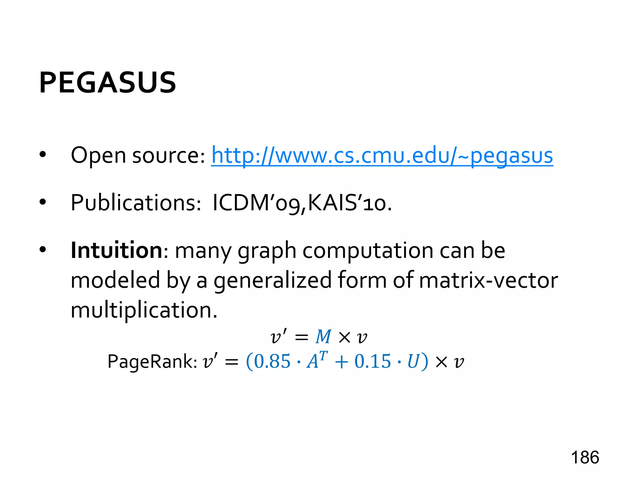


The document provides an overview of big graph analytics systems, covering various programming models, execution modes, and features of message passing systems like Google's Pregel. It discusses algorithms for graph problems, optimizations in communication mechanisms, and tools for out-of-core support and fault tolerance. Additionally, it examines different computation models, including block-centric computation and the performance of systems like Giraph and Blogel.


![[DSC Europe 25] Behzad Hosseini - AI Agents in the Wild: Deploying Models tha...](https://cdn.slidesharecdn.com/ss_thumbnails/3qtejajvsjqrzwfept2c-10-251212103250-7f2b1068-thumbnail.jpg?width=640&height=640&fit=bounds)
![[DSC Europe 25] Branko Urosevic -Rethinking Financial Talent: Integrating Cod...](https://cdn.slidesharecdn.com/ss_thumbnails/8jjrus8ttko6qj64f58f-3-251212103250-642c6374-thumbnail.jpg?width=640&height=640&fit=bounds)
![[DSC Europe 25] Debmalya Biswas - Agentification: the art of transforming man...](https://cdn.slidesharecdn.com/ss_thumbnails/r5azlggvtqiaiiusrqdr-4-251212103249-5a12c89b-thumbnail.jpg?width=640&height=640&fit=bounds)

![[DSC Europe 25] Kaja Kandare - LLM as a judge.pptx](https://cdn.slidesharecdn.com/ss_thumbnails/arxyccaxsdsd1ba99wjw-7-251212104007-2b4e3f64-thumbnail.jpg?width=640&height=640&fit=bounds)


![[DSC Europe 25] Bassam Maharmeh - Artificial Intelligence: Opportunities and ...](https://cdn.slidesharecdn.com/ss_thumbnails/thhfmr2fqpawzj7hsjpg-5-251211083048-2c23204f-thumbnail.jpg?width=640&height=640&fit=bounds)


![[DSC Europe 25] Jovan Bogicevic - Legacy to AI-Driven Defense: Transforming D...](https://cdn.slidesharecdn.com/ss_thumbnails/rsarluadt563hntyfc8q-3-251211083849-3e7bc4c0-thumbnail.jpg?width=640&height=640&fit=bounds)
![[DSC Europe 25] Dusan Nesic - Securing Tomorrow’s Infrastructure: Why Cyber-P...](https://cdn.slidesharecdn.com/ss_thumbnails/qikbszfftyowjm2q6duw-1-251211083848-8f2ead6b-thumbnail.jpg?width=640&height=640&fit=bounds)

![[DSC Europe 25] Nikolay Burlutskiy - Best Practices for Building Enterprise M...](https://cdn.slidesharecdn.com/ss_thumbnails/uirvaiuvq8y1w8hzd9tx-7-251212103249-2619edb4-thumbnail.jpg?width=640&height=640&fit=bounds)


![[DSC Europe 25] Dunja Adzic Jovanovic - AI and Cybersecurity: Defending Data ...](https://cdn.slidesharecdn.com/ss_thumbnails/o1zylpbhrtwnixxq2xj8-7-251211083048-185086f6-thumbnail.jpg?width=640&height=640&fit=bounds)