B10- ADVANCED FUNCTIONS OF MICROSOFT EXCEL.pptx

Data Analysis
using Microsoft
Excel

Recap
1 Introduction to excel
2
Sorting and Filtering techniques
3
Basic functions
(sum, avg, max, min, count etc.)

Agenda
Advanced Functions
(VLOOKUP, XlOOKUP, Match, Index)
Data Validation
Conditional Formatting
Pivot Tables and Pivot Charts

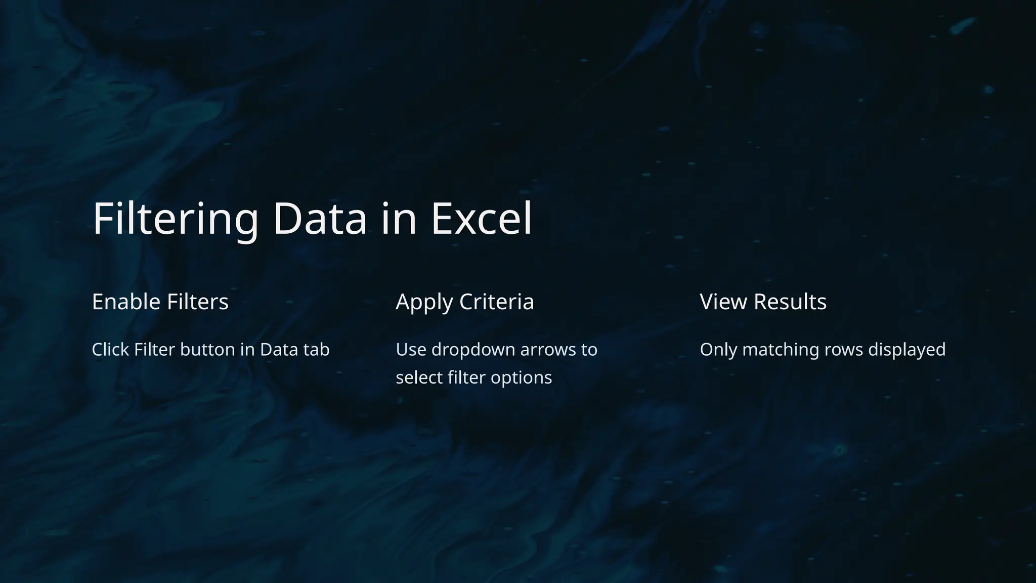
Filtering Data in Excel
Enable Filters
Click Filter button in Data tab
Apply Criteria
Use dropdown arrows to
select filter options
View Results
Only matching rows displayed

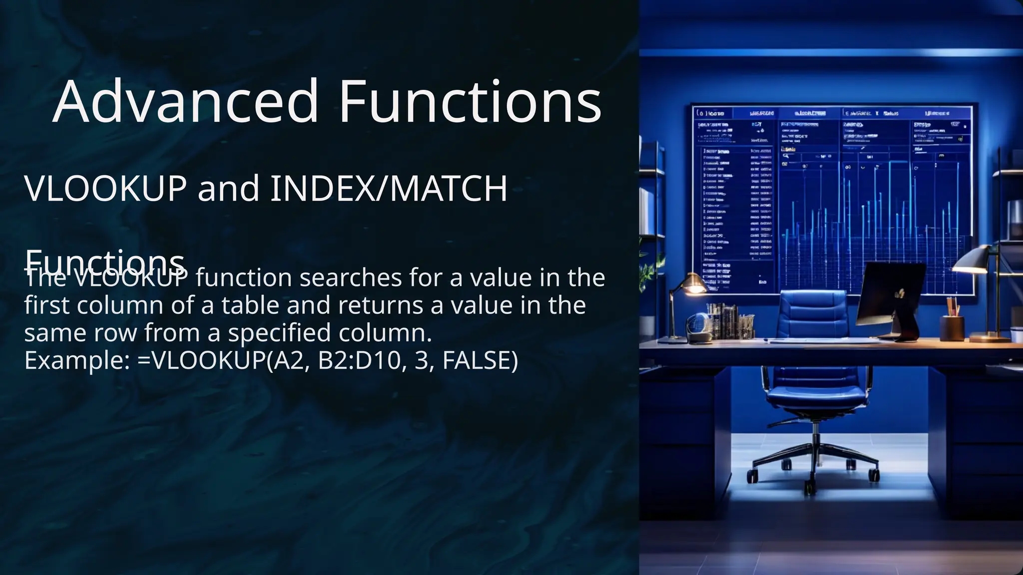
Advanced Functions
VLOOKUP and INDEX/MATCH
Functions
The VLOOKUP function searches for a value in the
first column of a table and returns a value in the
same row from a specified column.
Example: =VLOOKUP(A2, B2:D10, 3, FALSE)

Introduction to VLOOKUP
Definition
VLOOKUP is a powerful
function in Excel that
searches for a value in the
first column of a range
(table or array) and returns
a corresponding value in
the same row from a
specified column.
Syntax
=VLOOKUP(lookup_value,
table_array,
col_index_num,
[range_lookup])
Purpose
VLOOKUP is used to find
and retrieve specific data
from large datasets,
making it an essential tool
for data analysis and
reporting in Excel.

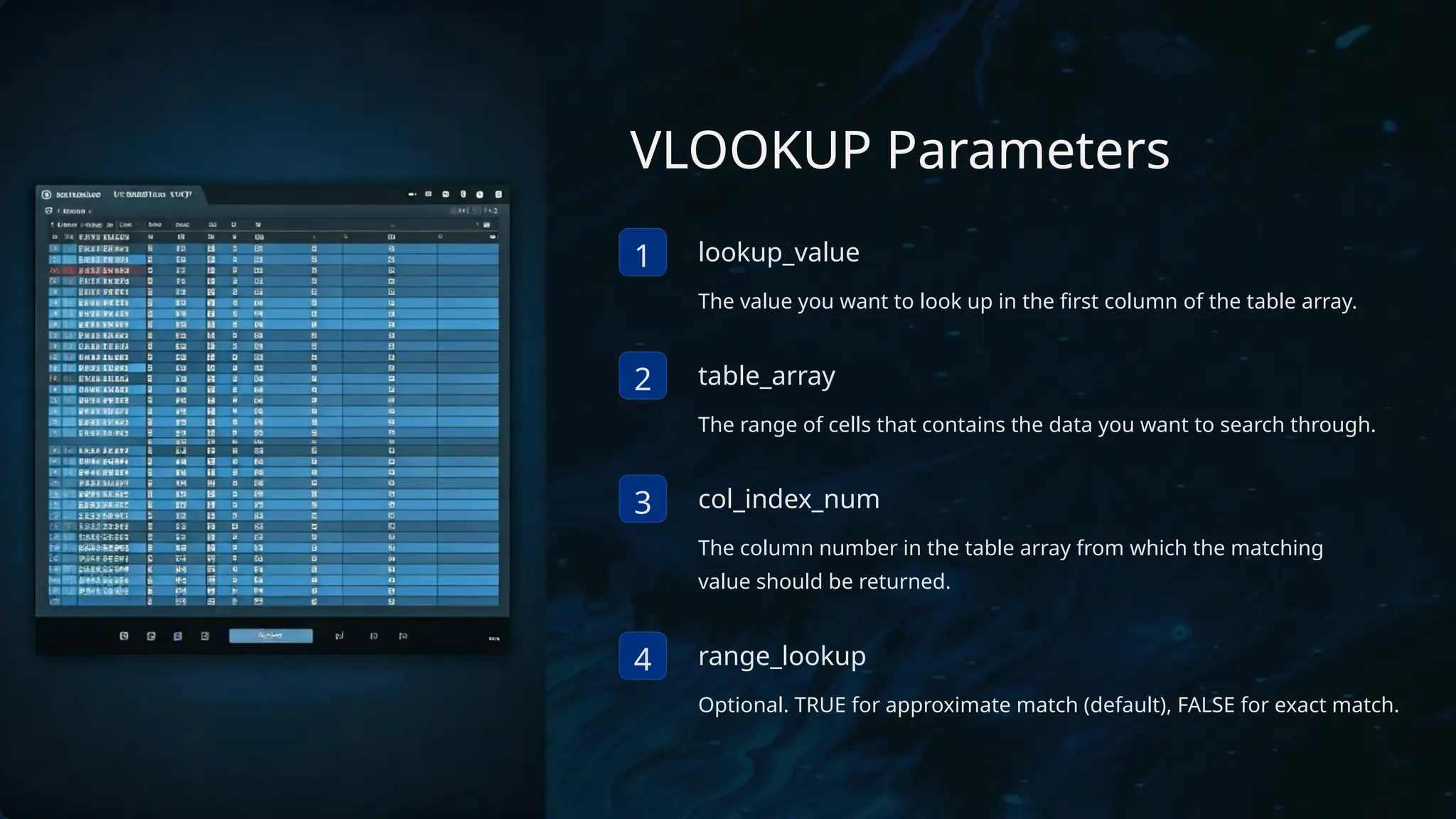
VLOOKUP Parameters
1 lookup_value
The value you want to look up in the first column of the table array.
2 table_array
The range of cells that contains the data you want to search through.
3 col_index_num
The column number in the table array from which the matching
value should be returned.
4 range_lookup
Optional. TRUE for approximate match (default), FALSE for exact match.

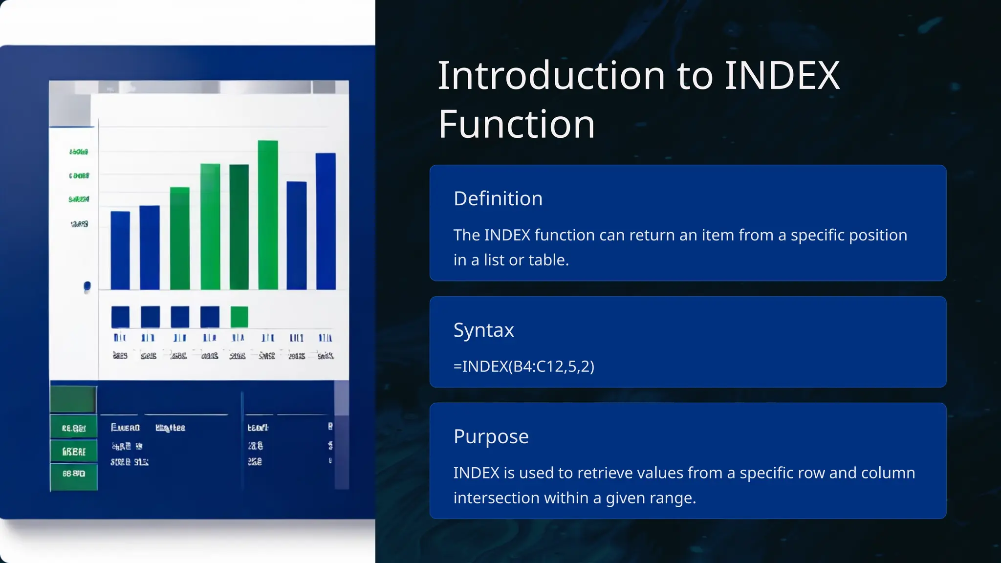
Introduction to INDEX
Function
Definition
The INDEX function can return an item from a specific position
in a list or table.
Syntax
=INDEX(B4:C12,5,2)
Purpose
INDEX is used to retrieve values from a specific row and column
intersection within a given range.

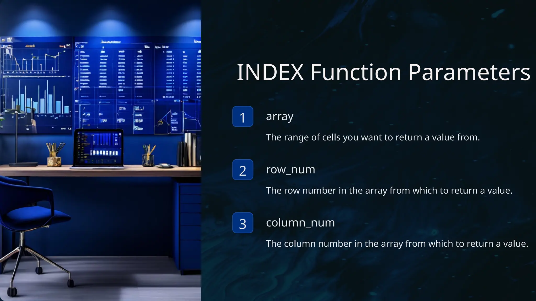
INDEX Function Parameters
1 array
The range of cells you want to return a value from.
2 row_num
The row number in the array from which to return a value.
3 column_num
The column number in the array from which to return a value.

Introduction to MATCH
Function
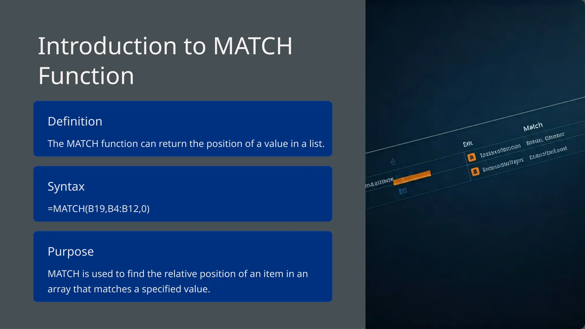
Definition
The MATCH function can return the position of a value in a list.
Syntax
=MATCH(B19,B4:B12,0)
Purpose
MATCH is used to find the relative position of an item in an
array that matches a specified value.

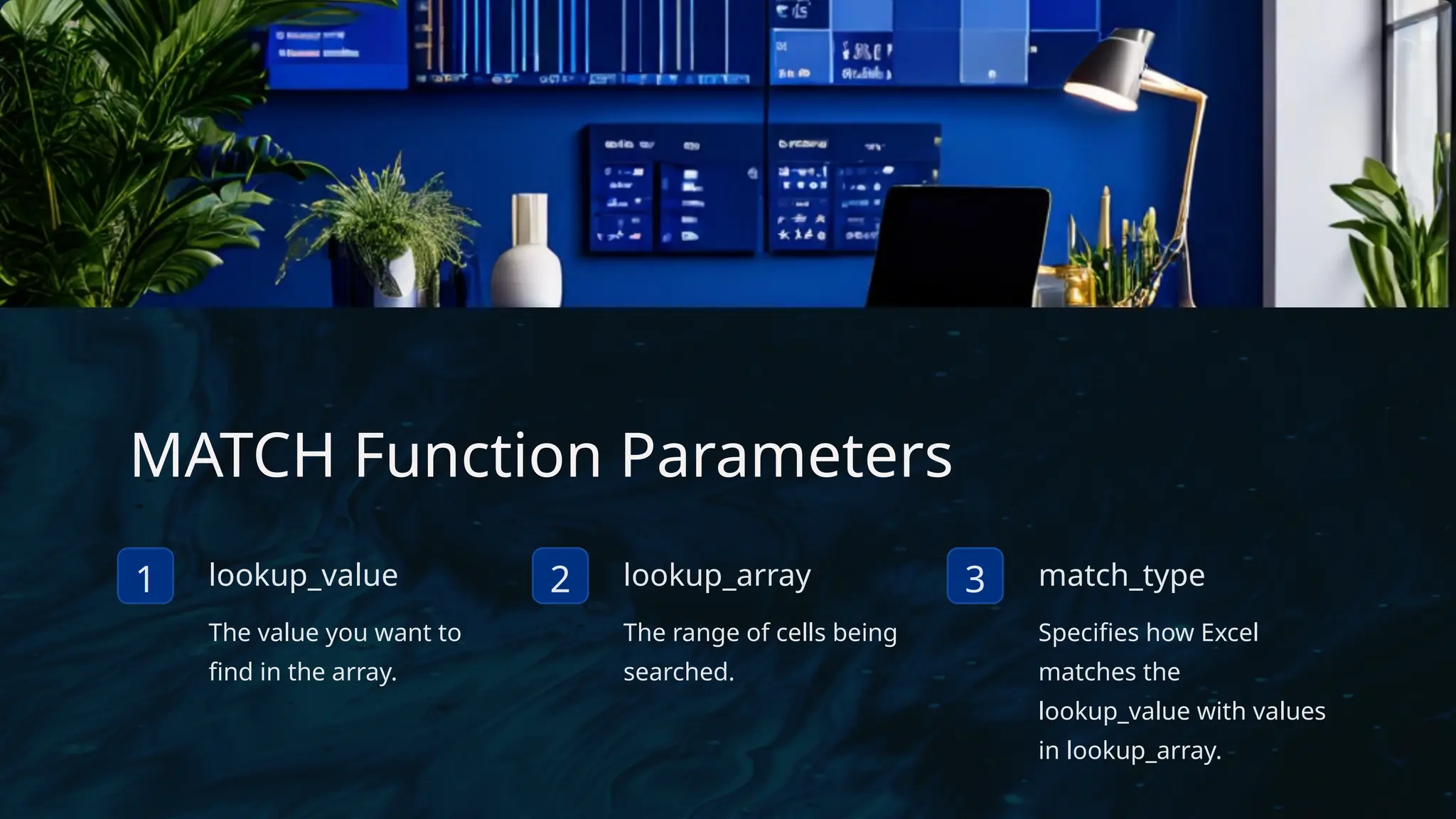
MATCH Function Parameters
1 lookup_value
The value you want to
find in the array.
2 lookup_array
The range of cells being
searched.
3 match_type
Specifies how Excel
matches the
lookup_value with values
in lookup_array.

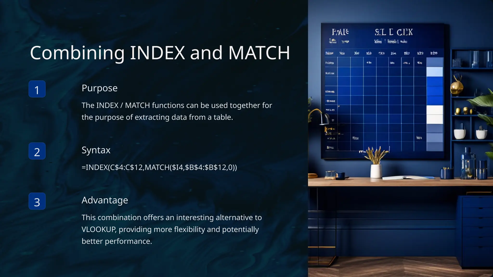
Combining INDEX and MATCH
1 Purpose
The INDEX / MATCH functions can be used together for
the purpose of extracting data from a table.
2 Syntax
=INDEX(C$4:C$12,MATCH($I4,$B$4:$B$12,0))
3 Advantage
This combination offers an interesting alternative to
VLOOKUP, providing more flexibility and potentially
better performance.

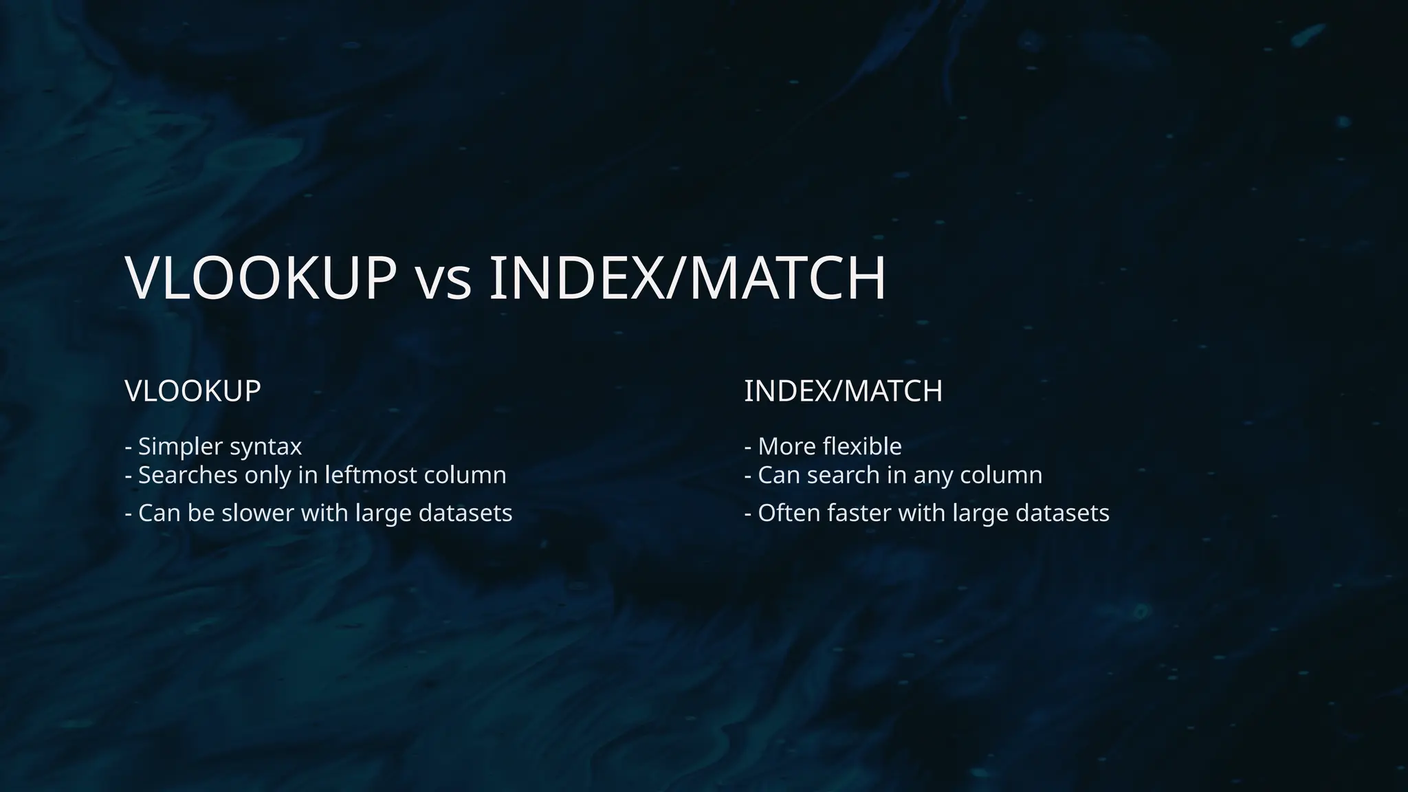
VLOOKUP vs INDEX/MATCH
VLOOKUP
- Simpler syntax
- Searches only in leftmost column
- Can be slower with large datasets
INDEX/MATCH
- More flexible
- Can search in any column
- Often faster with large datasets

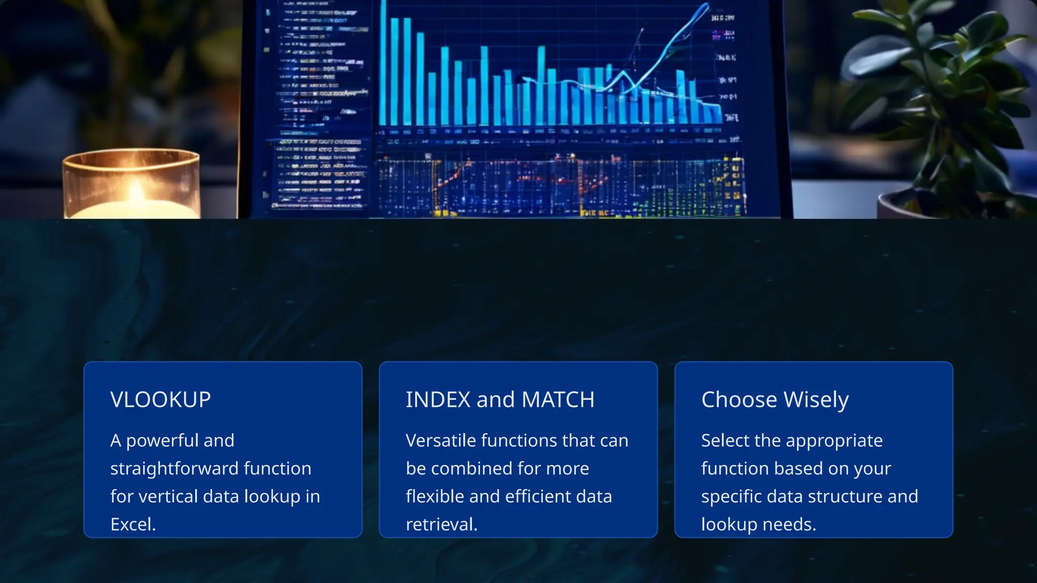
VLOOKUP
A powerful and
straightforward function
for vertical data lookup in
Excel.
INDEX and MATCH
Versatile functions that can
be combined for more
flexible and efficient data
retrieval.
Choose Wisely
Select the appropriate
function based on your
specific data structure and
lookup needs.

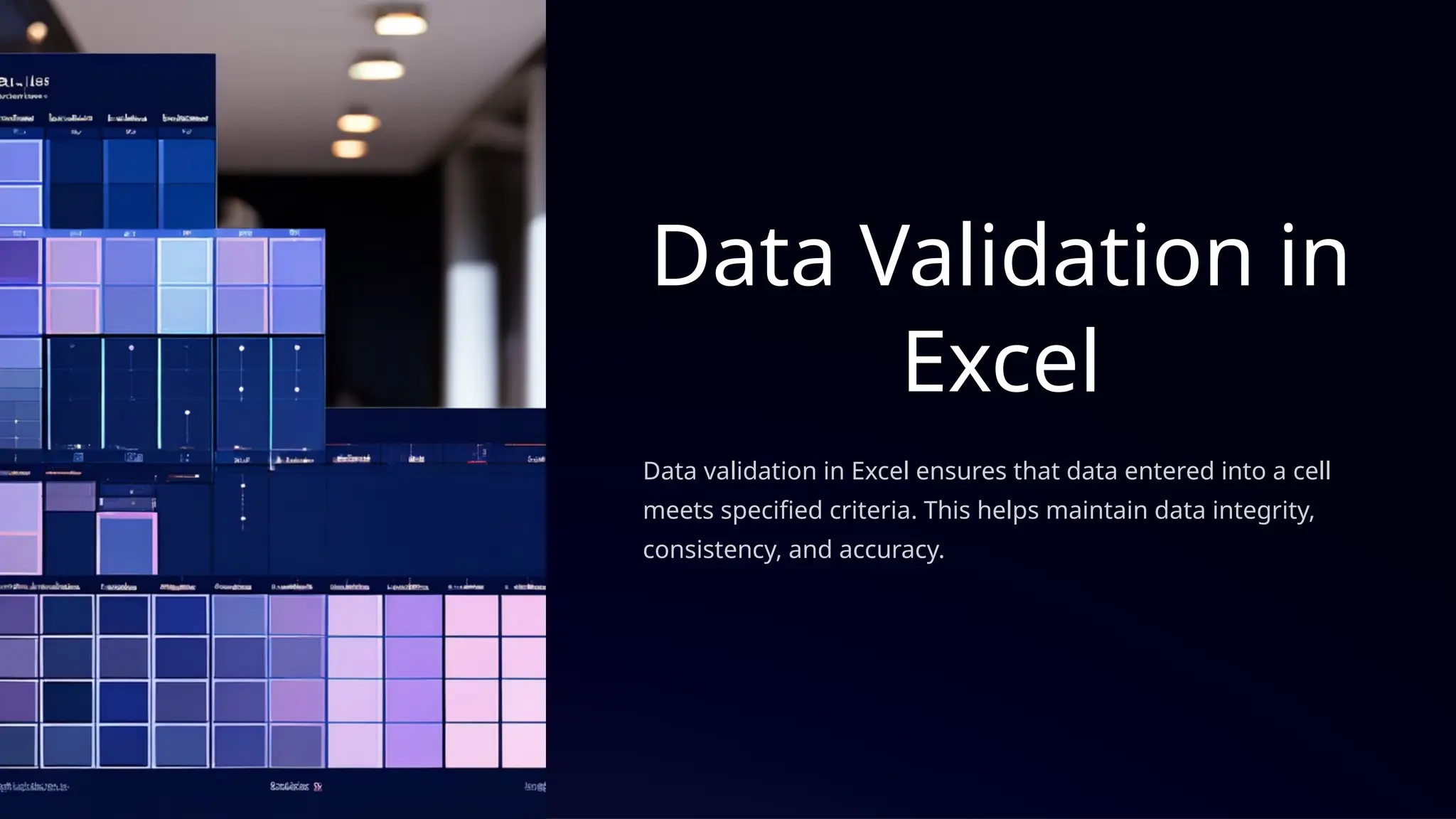
Data Validation in
Excel
Data validation in Excel ensures that data entered into a cell
meets specified criteria. This helps maintain data integrity,
consistency, and accuracy.

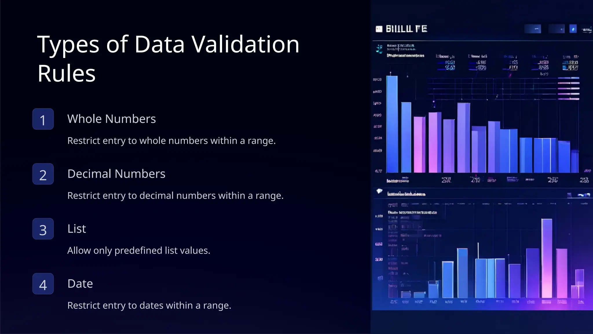
Types of Data Validation
Rules
1 Whole Numbers
Restrict entry to whole numbers within a range.
2 Decimal Numbers
Restrict entry to decimal numbers within a range.
3 List
Allow only predefined list values.
4 Date
Restrict entry to dates within a range.

Input Messages and Error Alerts
Input Message
Provides guidance when a cell is selected.
Error Alert Types
• Stop
• Warning
• Information

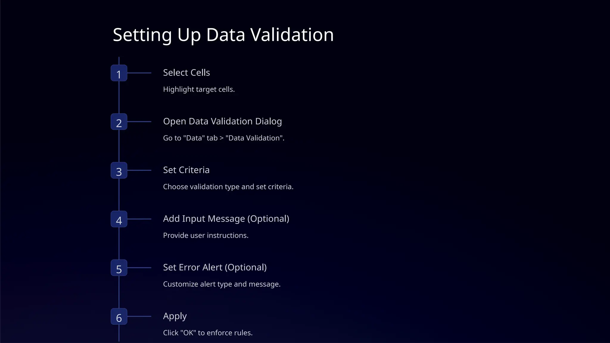
Setting Up Data Validation
1 Select Cells
Highlight target cells.
2 Open Data Validation Dialog
Go to "Data" tab > "Data Validation".
3 Set Criteria
Choose validation type and set criteria.
4 Add Input Message (Optional)
Provide user instructions.
5 Set Error Alert (Optional)
Customize alert type and message.
6 Apply
Click "OK" to enforce rules.

Introduction to
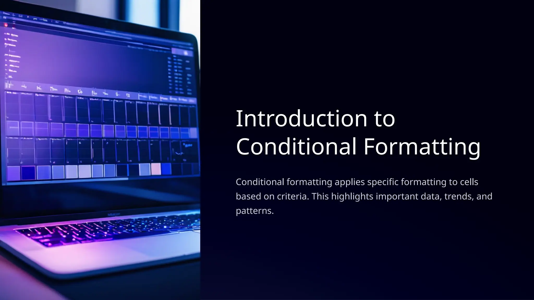
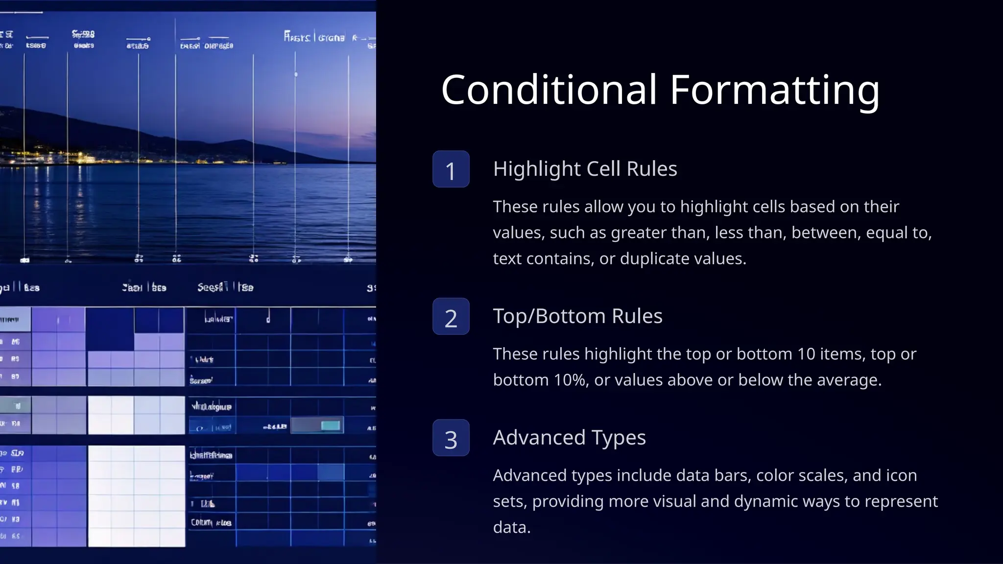
Conditional formatting applies specific formatting to cells
based on criteria. This highlights important data, trends, and
patterns.

1 Highlight Cell Rules
These rules allow you to highlight cells based on their
values, such as greater than, less than, between, equal to,
text contains, or duplicate values.
2 Top/Bottom Rules
These rules highlight the top or bottom 10 items, top or
bottom 10%, or values above or below the average.
3 Advanced Types
Advanced types include data bars, color scales, and icon
sets, providing more visual and dynamic ways to represent
data.

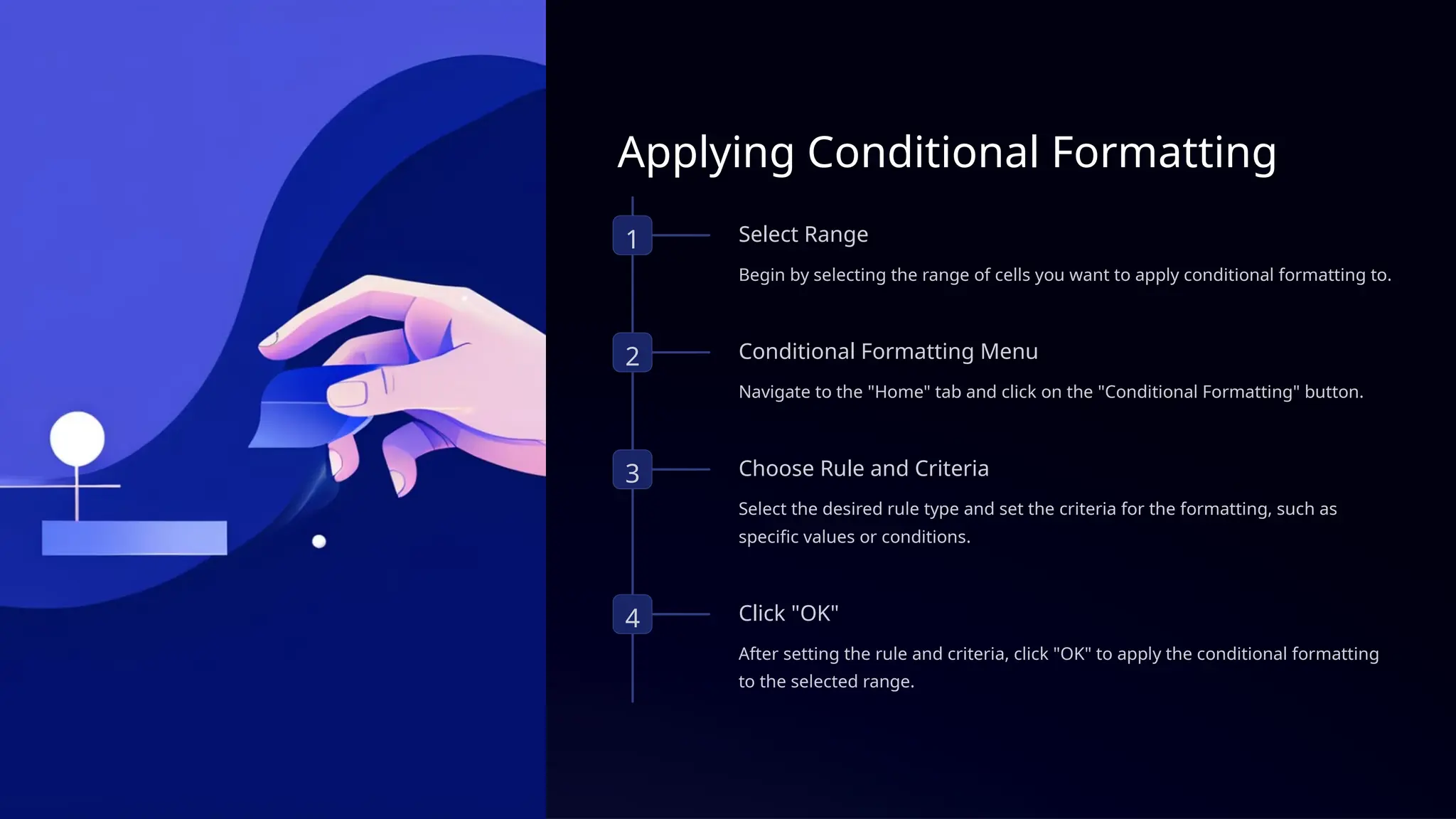
Applying Conditional Formatting
1 Select Range
Begin by selecting the range of cells you want to apply conditional formatting to.
2 Conditional Formatting Menu
Navigate to the "Home" tab and click on the "Conditional Formatting" button.
3 Choose Rule and Criteria
Select the desired rule type and set the criteria for the formatting, such as
specific values or conditions.
4 Click "OK"
After setting the rule and criteria, click "OK" to apply the conditional formatting
to the selected range.

Introduction to Pivot
Tables
A Pivot Table in Excel is a powerful tool used to summarize,
analyze, and explore large datasets by reorganizing and
grouping data. It allows users to quickly create reports by
dragging and dropping fields to calculate sums, averages,
counts, and more without altering the original data. Pivot
Tables are ideal for dynamically exploring trends and patterns
in data.

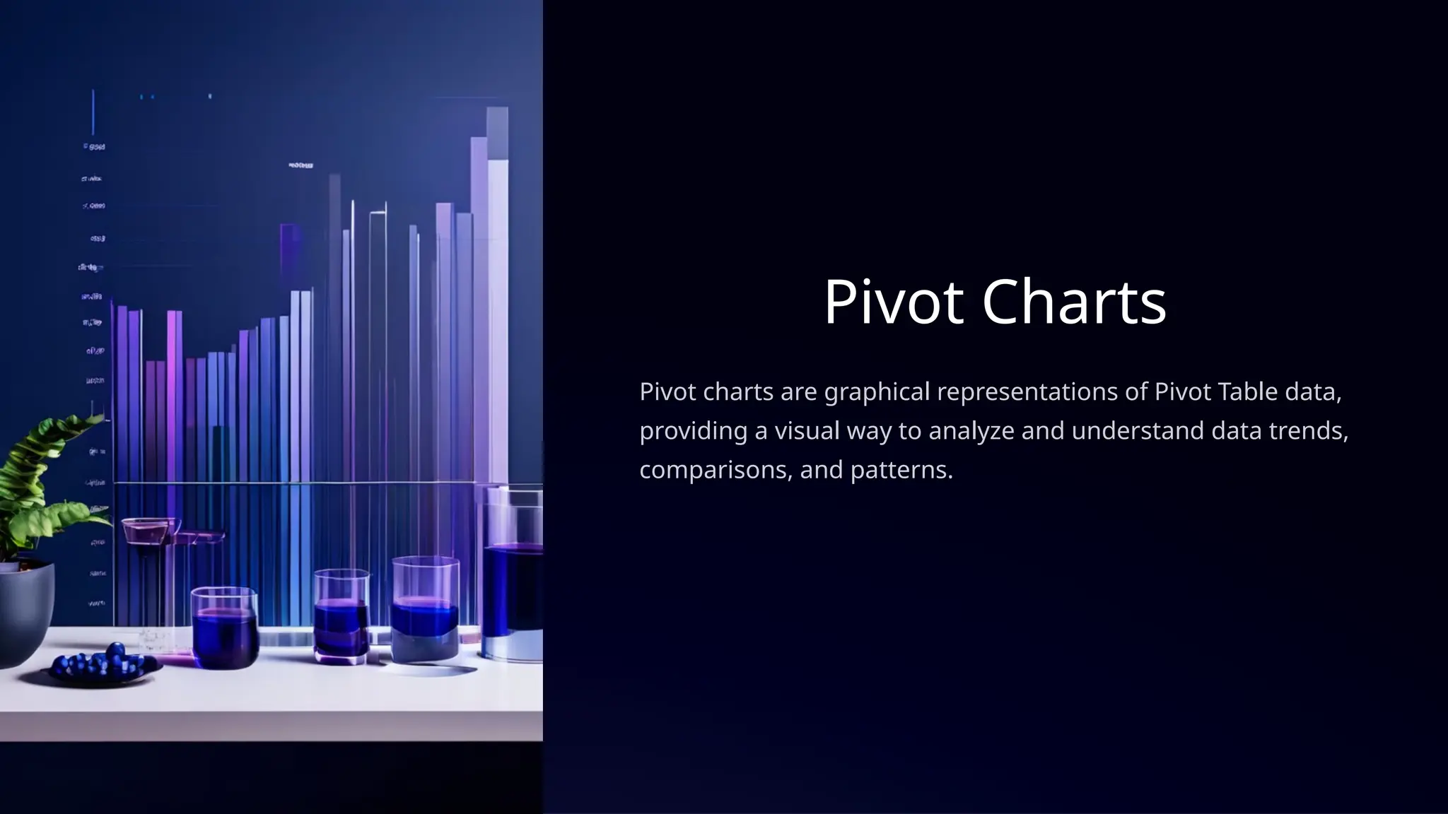
Pivot Charts
Pivot charts are graphical representations of Pivot Table data,
providing a visual way to analyze and understand data trends,
comparisons, and patterns.

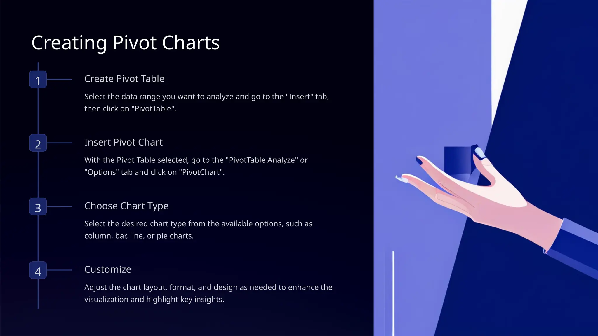
Creating Pivot Charts
1 Create Pivot Table
Select the data range you want to analyze and go to the "Insert" tab,
then click on "PivotTable".
2 Insert Pivot Chart
With the Pivot Table selected, go to the "PivotTable Analyze" or
"Options" tab and click on "PivotChart".
3 Choose Chart Type
Select the desired chart type from the available options, such as
column, bar, line, or pie charts.
4 Customize
Adjust the chart layout, format, and design as needed to enhance the
visualization and highlight key insights.

Benefits and Usage of Pivot Charts
Interactive Analysis
Pivot charts allow for dynamic
data exploration through filters
and slicers, enabling you to
quickly analyze different
aspects of the data.
Data Summarization
They provide a quick and easy
way to summarize large
datasets, presenting key
insights in a visually appealing
and understandable format.
Trend Identification
Pivot charts help you easily
spot trends, outliers, and
patterns in the data, making it
easier to identify key insights
and make informed decisions.

B10- ADVANCED FUNCTIONS OF MICROSOFT EXCEL.pptx

More Related Content

Similar to B10- ADVANCED FUNCTIONS OF MICROSOFT EXCEL.pptx

More from Atoshe Elmi

Recently uploaded

B10- ADVANCED FUNCTIONS OF MICROSOFT EXCEL.pptx