En premier lieu, je tiensà remercier de tout coeur ma directrice de thèse, Nicole El Karoui, pour la qualité exceptionnelle de son encadrement. Son savoir, son dynamisme et sa rigueur ont fortement contribuéà la rédaction de cette thèse....
moreEn premier lieu, je tiensà remercier de tout coeur ma directrice de thèse, Nicole El Karoui, pour la qualité exceptionnelle de son encadrement. Son savoir, son dynamisme et sa rigueur ont fortement contribuéà la rédaction de cette thèse. C'était un grand honneur d'avoir découvert le monde de la rechercheà ses côtés : elle m'a donné le goût de la recherche en me transmettant sa passion. J'admire son savoir immense mais je pense que j'admire encore plus ses qualités humaines. Nicole a toujoursété disponible pour moi et a réponduà toutes mes questions avec gentillesse et enthousiasme. Je lui suis vraiment reconnaissant pour le soutien et la confiance qu'elle m'a accordé. Mes remerciements respectueuxà Jean Pierre Fouque et Christian Gourieroux de m'avoir fait l'honneur de rapporter ma thèse. Ils m'ont envoyé de nombreuses corrections et un ensemble de conseils précieux qui m'ont permis d'améliorer la rédaction. Je présente mes sincères remerciementsà Sylvie Méléard, Christophe Michel, Nizar Touzi et Alain Trognon de m'avoir fait l'honneur d'accepter de participerà mon jury de thèse. Je tiensà remercier particulièrement Christophe Michel qui m'a accueilli pendant trois années dans sonéquipe de recherche du Crédit Agricole et qui m'a suivi, aidé et conseillé tout au long de cette thèse. Je remercie aussi Anas, membre de l'équipe, d'avoir partagé de nombreuses connaissances et d'avoir accepté de rédiger des articles ensemble. Je remercie Florence pour l'aideà la relecture de la thèse et je remercie vivement Vincent pour ses nombreux conseils avisés et son aide précieuse. Enfin, je remercie toute l'équipe de recherche de CA-CIB pour son accueil chaleureux, et plus particulièrement Vincent, Sophie, Christophe M. et Christophe Z., Kenza, Florence, Thomas, Eric avec qui j'ai pu tisser des liens d'amitié. Mes remerciements d'adressentégalement aux membres du groupe de longévité et plus particulièrement Caroline Hillairet, Stéphane Loisel, Yahia Salhi, Pauline Barrieu, Isabelle Camillier et Trung Lap NGuyen. Ces réunions ontété très enrichissantes et nous avons pu travailler ensemble et partager des discussions sur de nombreux sujets passionnants. Je remercie vivement Chi Tran Viet et Sylvie Méléard pour m'avoir aidéà me plonger dans le domaine de la dynamique de population. Chi m'a aidéà de nombreuses reprises en répondantà mes questions et en me fournissant des pistes de réflexion très intéressantes. Je remercie aussi les membres du groupe de travail de biologie de l'école polytechnique. Un grand mercià Martino Grasseli et José Da Fonseca pour les nombreux conseils qu'ils m'ont donné sur les modèles de Wishart et pour l'intérêt qu'ils ont montré sur mes travaux de recherche. i Je pense aussi aux doctorants du CMAP, et en particulierà Gilles-Edouard, Emilie, Laurent, Isabelle, Mohammed et Trunglap ainsi qu'à l'ensemble des chercheurs du CMAP avec lesquels j'ai pu partager des moments privilégiés. Je pense en particulierà Peter, Emmanuel et Nizar qui ontété disponible et m'ont donné des conseils précieux. Merci au personnel administratif du CMAP, en particulierà Nassera, Anna, Sandra, Nathalie et Alexandra, pour leur gentillesse et leur aide dans leur bonne humeur. Je remercie aussi l'administrateur informatique Sylvain de son assistance ainsi qu'à Aldjia pour m'avoir aidé dans de nombreuses démarches. Enfin, je penseà l'ensemble des membres de l'école doctorale et en particulier Audrey et Fabrice qui m'ont aidé dans toutes les démarches. Je voudrais remercier tous mes amis proches qui ont contribuéà monépanouissement. Mercì a Dany, mon "colloc" adoré avec qui j'ai passé une année géniale, mes "petites soeurs" Cynthia et Karen et l'ensemble de mes amis proches

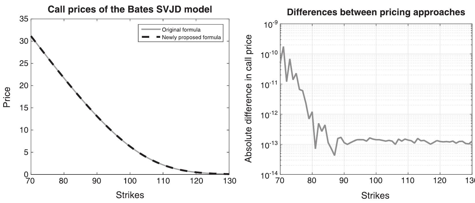
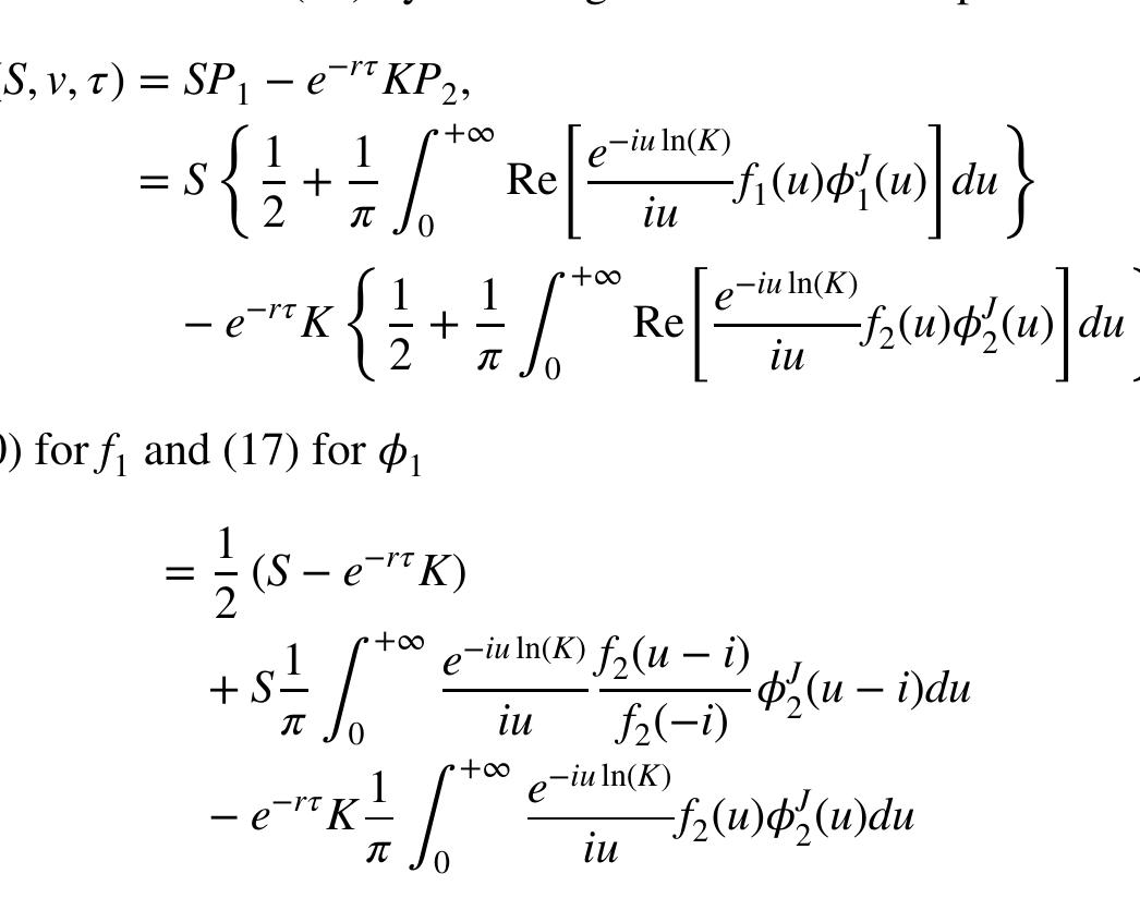
![As mentioned before, there exist many different formulas, for example, by Kahl and Jackel [28], Lewis[29] or Zhylyevskyy [36]. We will use the approach by Lewis [29] because it is well suited for more complex models with jumps. It is also well behaved compared with the formula by Albrecher et al. [27] but has the numerical advantage that we only have to calculate one integral for each call option price. where X = In(S/K) + rr and](https://figures.academia-assets.com/118628658/figure_001.jpg)
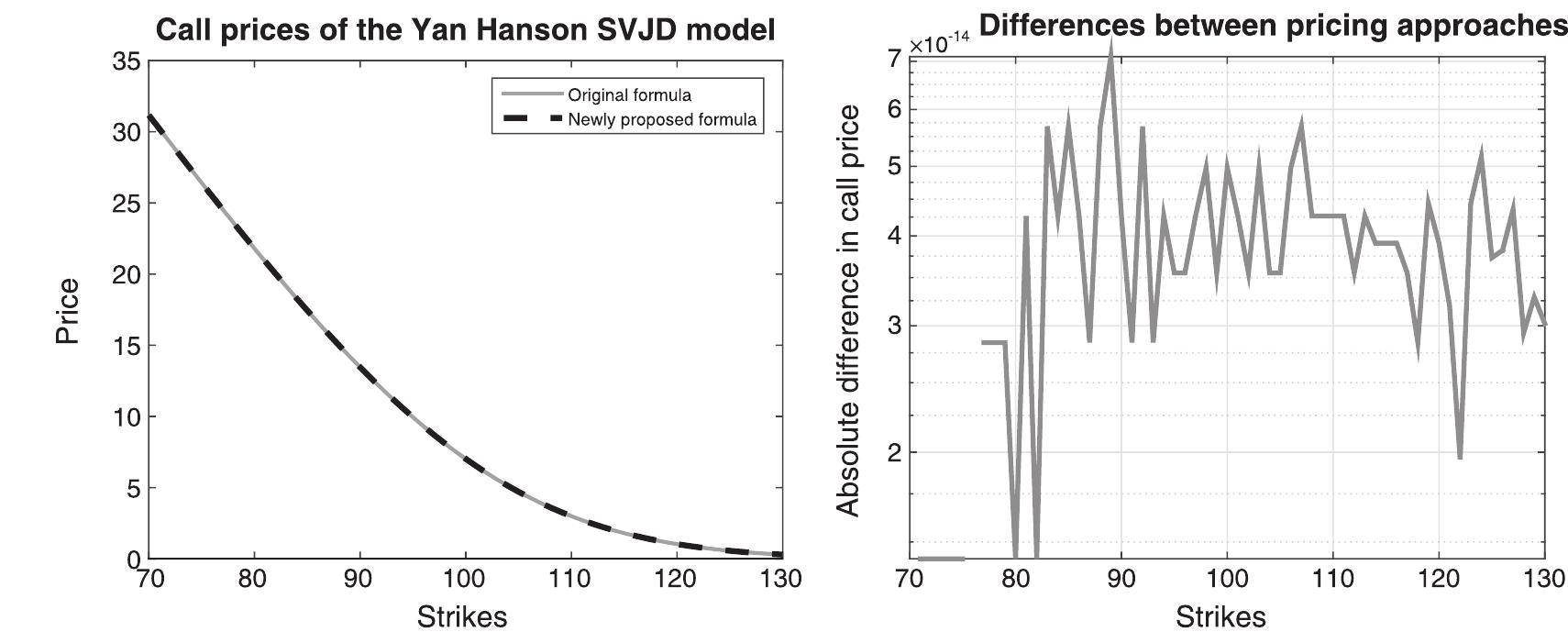
![New pricing formula for the Yan Hanson model is (31) with otk) defined in (23), or (33) in terms of @(k). 4.2. Example: a new fractional SVJD model We want to modify the Bates model from Section 3 by using an approximate fractional Brownian motion in the volatility process. This process has a long memory for Hurst parameter H > 0.5, and for H = 0.5, it turns into a standard Wiener process. Thao [39] defined approximative fractional process as an It6 integral,](https://figures.academia-assets.com/118628658/figure_014.jpg)
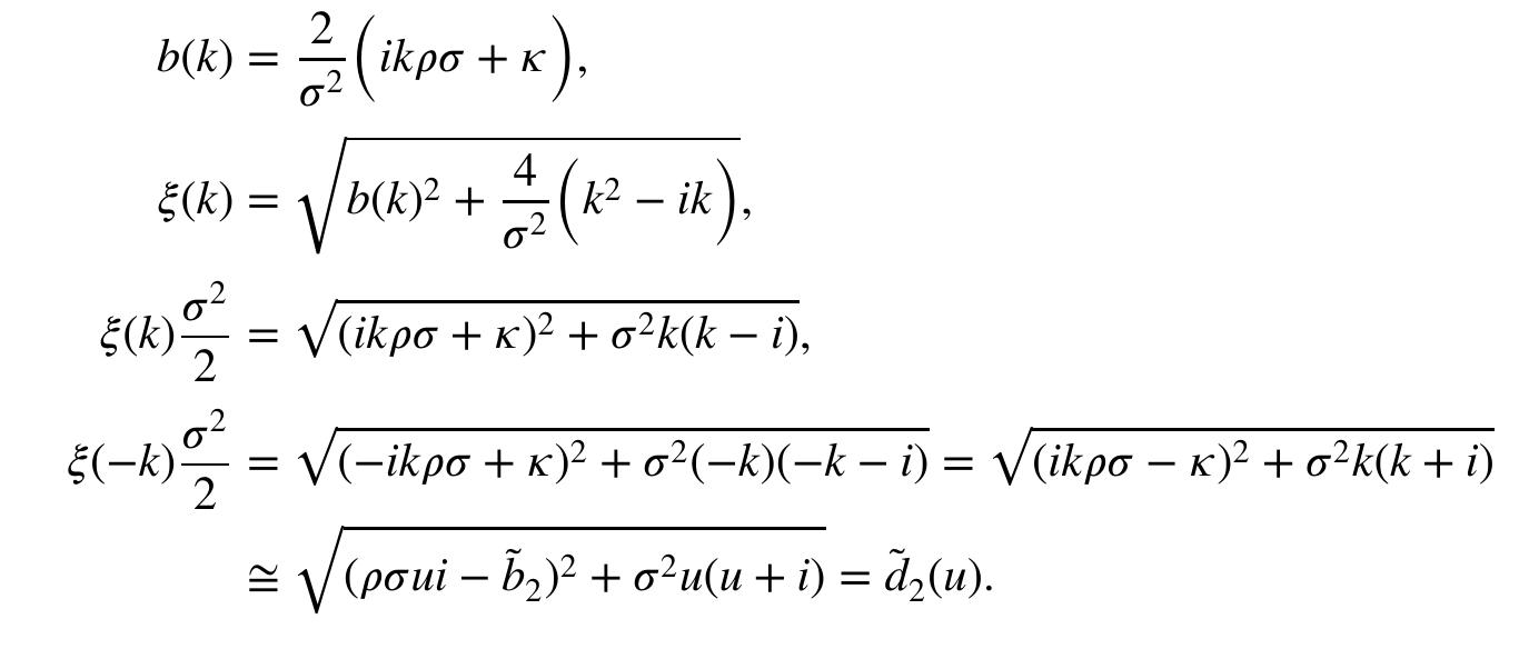
![where (W,),59 is a standard Wiener process, p < 0, A, vy 2 0 and (Z,),50 is a Lévy subordinator (independent on W,)!!. The model price of a call option with strike K can be retrieved using a standard Fourier transform [17]. Option price (A3) can be rewritten using the notation C(u) = C(u, tT) = exp{A(u, tT) + B(u, r)}. Also, note that C(—i) = 1 for any positive tT.](https://figures.academia-assets.com/118628658/figure_019.jpg)
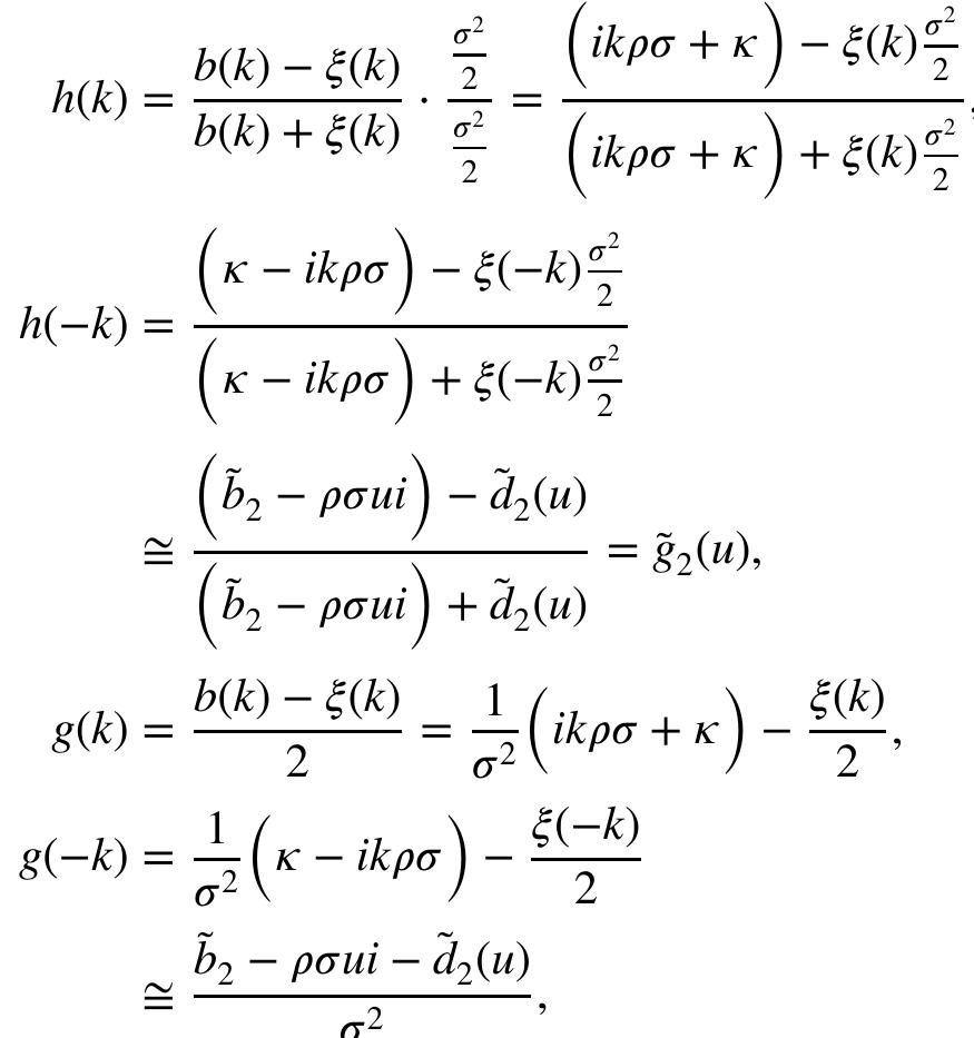
![where we used the Fubini’s theorem (the integrand is measurable and integrable) and the fact that ie g(y)dy = 1. W substitute t = T — t and define h(k, v, t) by to obtain from (25) the following equation for h: which is equal to equation (2.7) on p. 38 in Lewis [29] and has a fundamental solution F with initial value F (k,v,0) = 1 (in Lewis [29], it is called fundamental transform). It is regular as a function of k = k, + ik; within a strip k,; < k; < kp. From this fundamental solution, we can derive the explicit formula for the option price](https://figures.academia-assets.com/118628658/figure_013.jpg)
![and @(k) is defined in (32) with @(k) as in Example |. Similarly, we could use the formula (31). Equation (41) is a Ricatti equation and can be solved explicitly (for example, PospiSil and Sobotka [26], Proposition 2.1), and then we obtain C; by integrating (42). The formula (33) for this model with approximate fractional Brownian motion is](https://figures.academia-assets.com/118628658/figure_015.jpg)
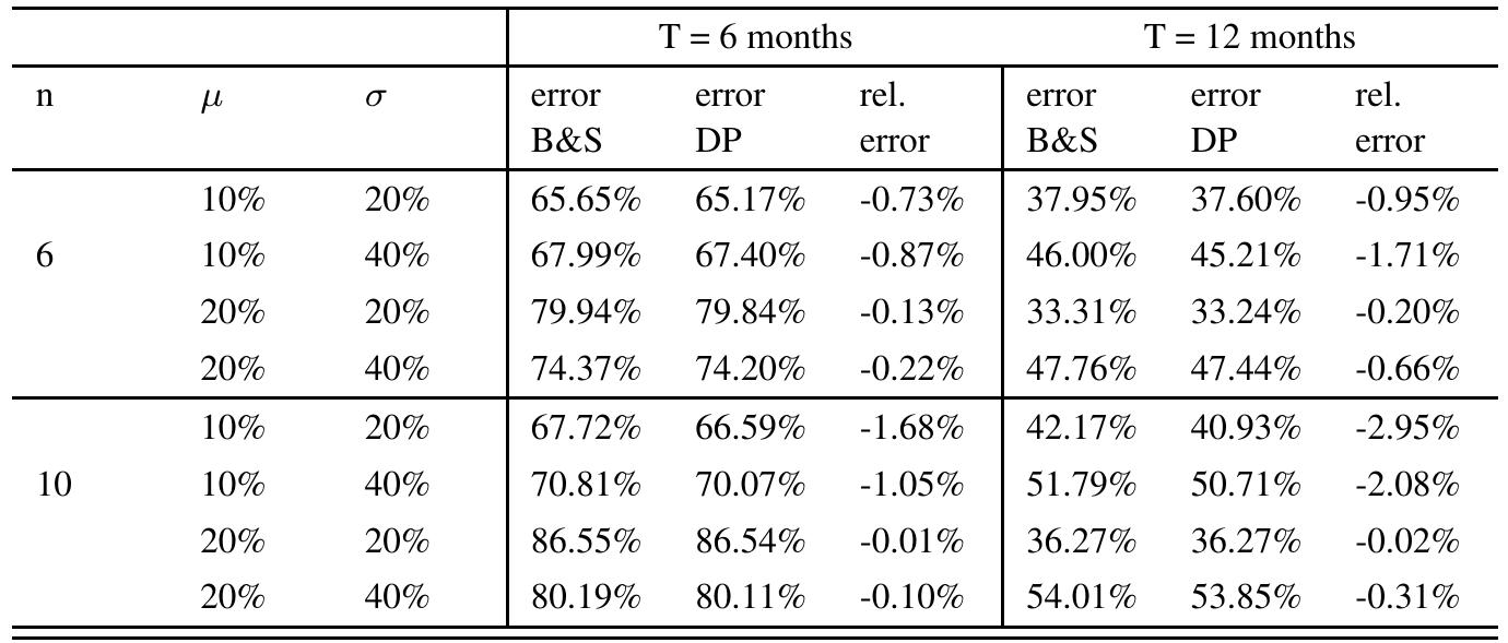
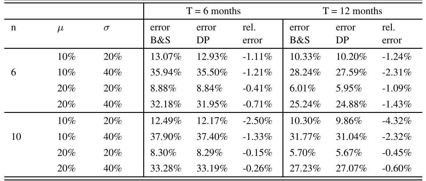
![Extending the work of Cerny [1] to the case where the price of a risky asset price is represented by a lognormal geometric brownian motion with constant parameters, as in (2.2), we obtain explicit expressions for both the mean-value process, H(r), of the option to be hedged, and the optimal control, u(r), to be applied at the rebalancing instant 7. The main results are given by Theorems 2.1 and 2.2 stated below. Full proofs can be found in Maiali [6]. In what follows we use the following notation:](https://figures.academia-assets.com/105324473/figure_001.jpg)