Neutrosophic Stable Random Variables

Neutrosophic Sets and Systems, Vol. 50, 2022 University of New Mexico Neutrosophic Stable Random Variables Azzam Mustafa Nouri 1, Omar Zeitouny 2 and Sadeddin Alabdallah 3,* 1 Department of Mathematical Statistics, University of Aleppo, Aleppo, Syria; [email protected]. 2 Department of Mathematical Statistics, University of Aleppo, Aleppo, Syria; [email protected]. 3 Department of Mathematical Statistics, University of Aleppo, Aleppo, Syria; [email protected]. 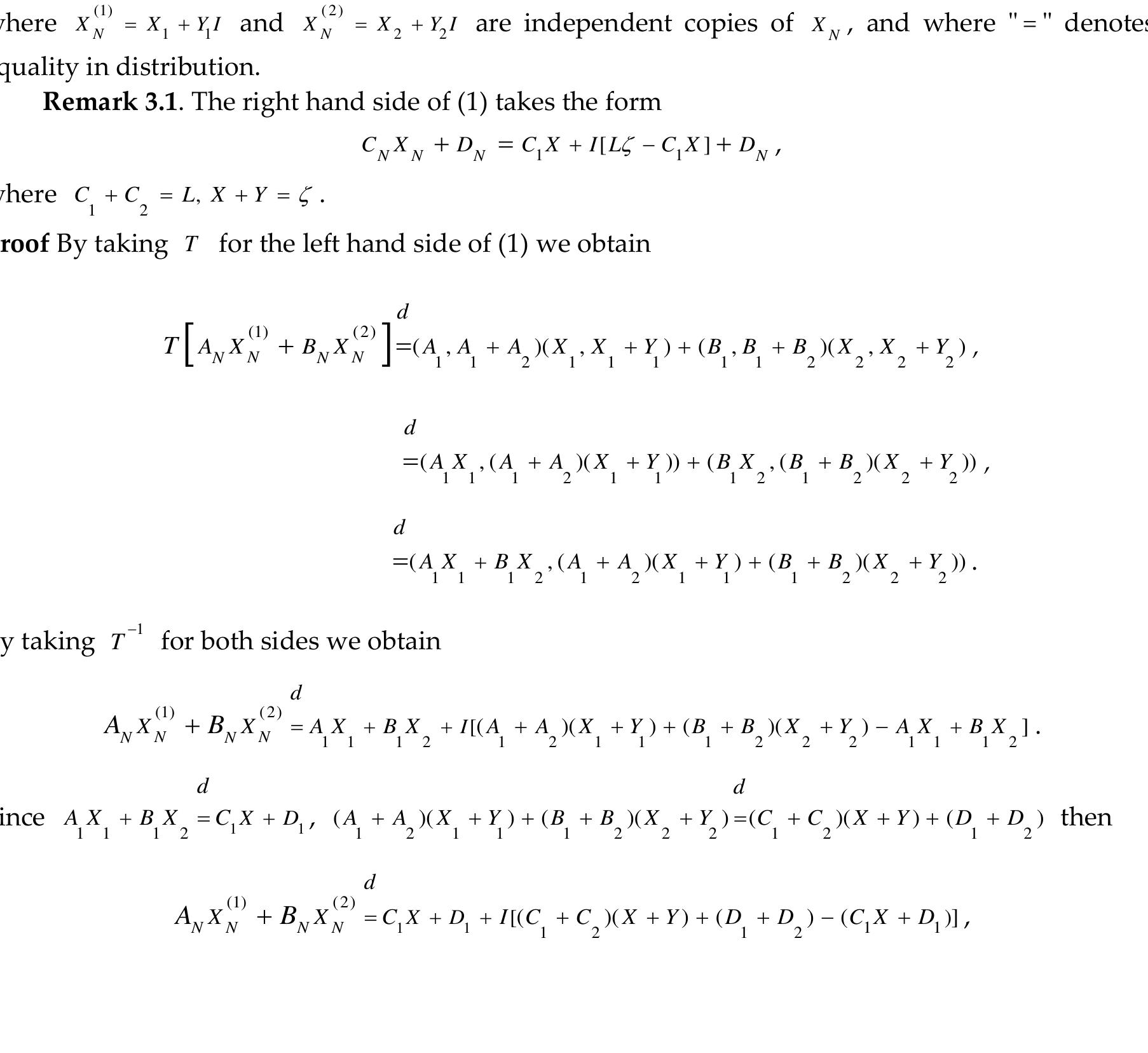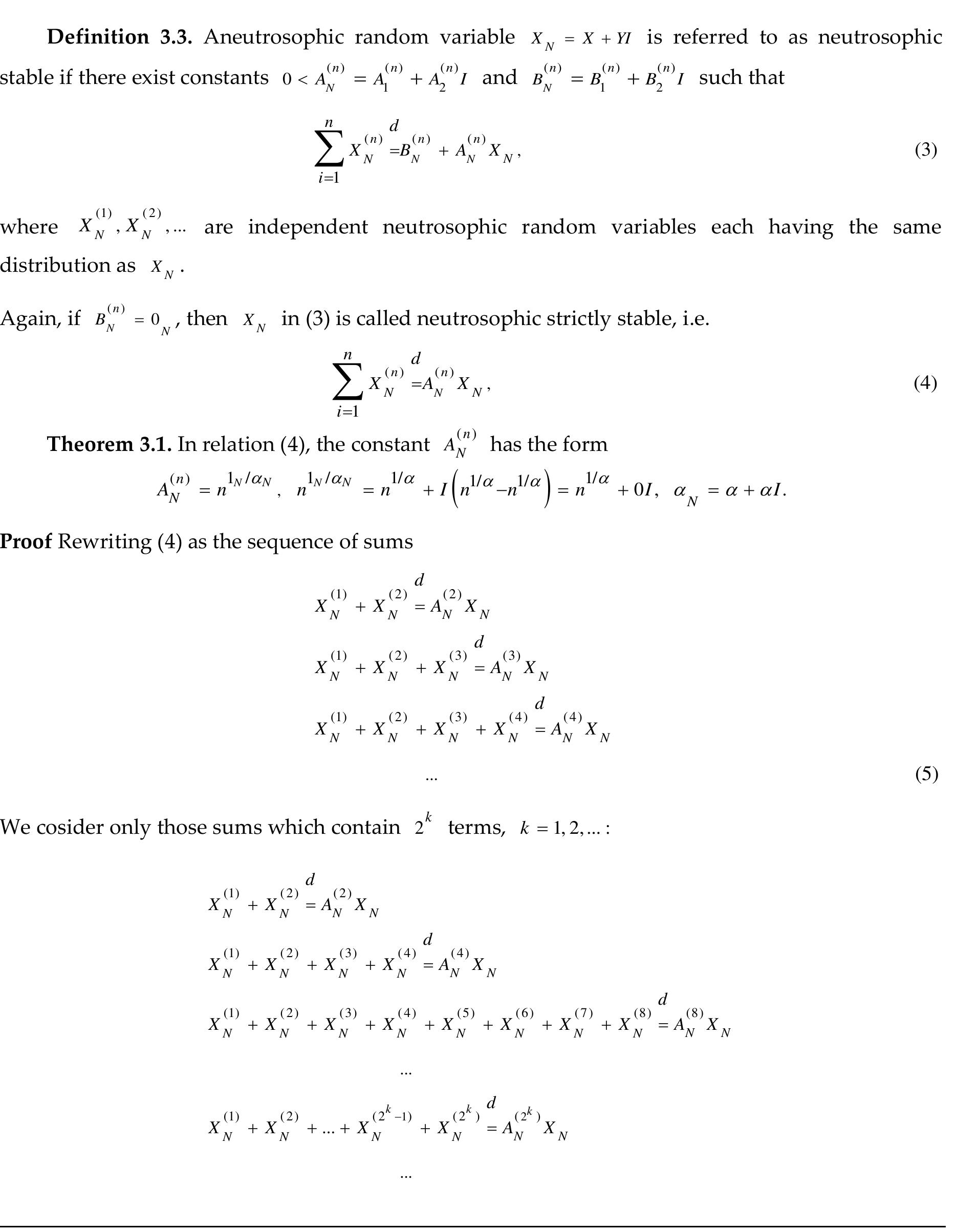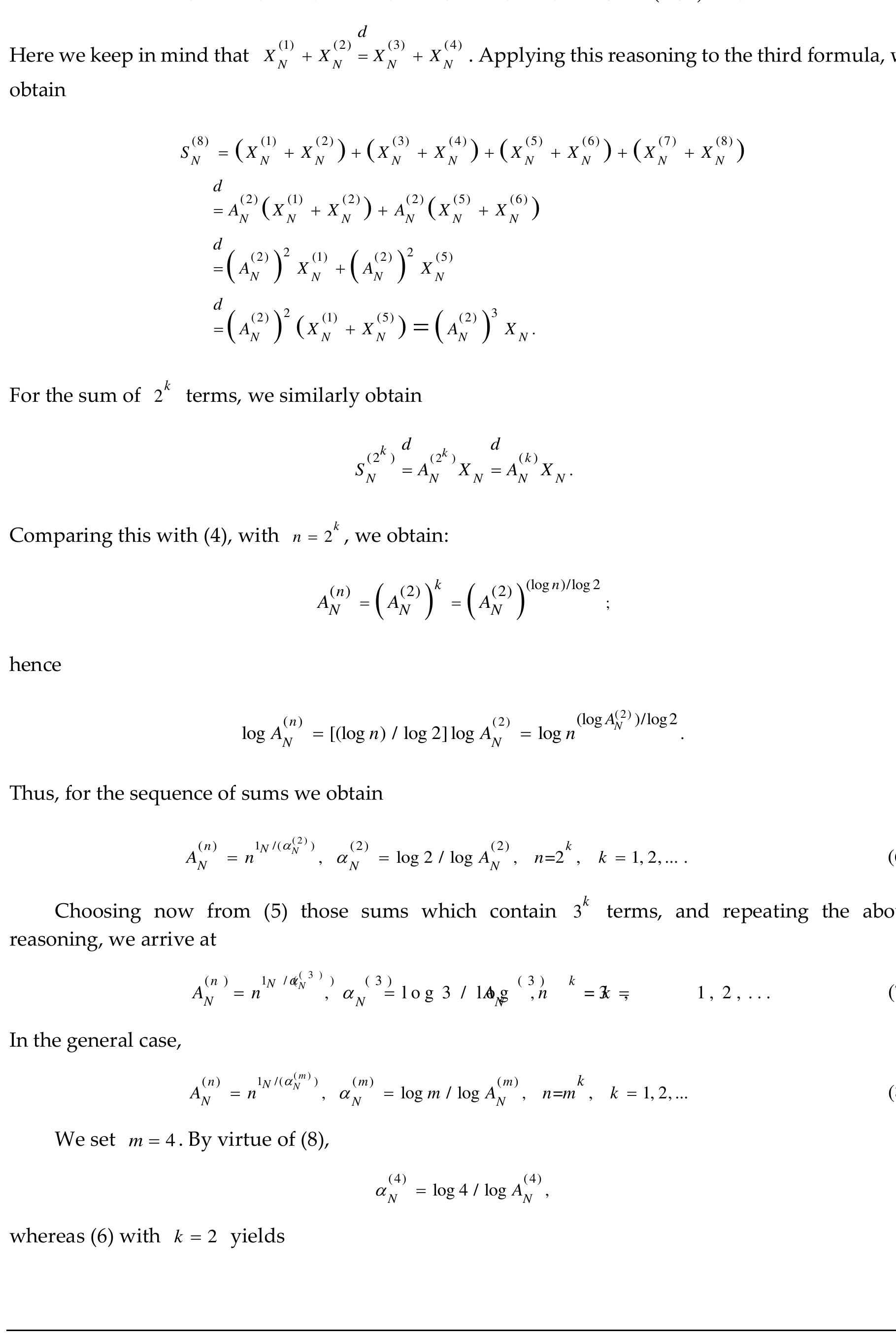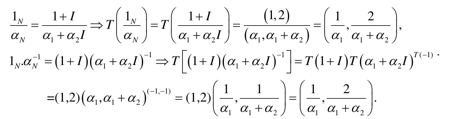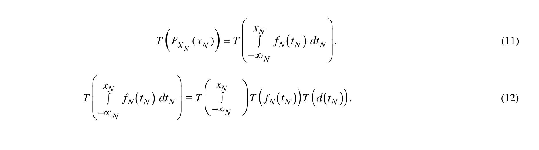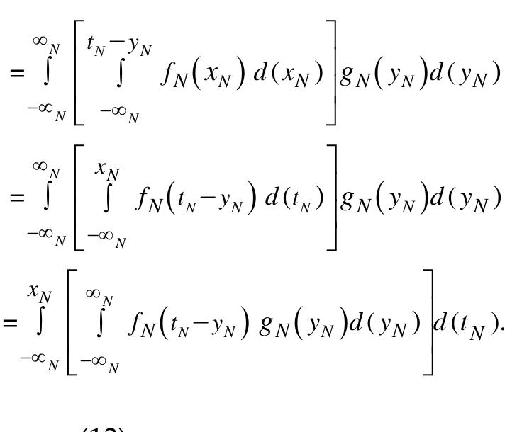* Correspondence: [email protected]; Tel.: (00963941339816) Abstract: In this paper, the concept of a neutrosophic stable random variable is introduced. Two definitions of a neutrosophic random variable are presented. We introduced both the neutrosophic probability distribution function and the neutrosophic probability density function, and the convolution with the neutrosophic concept. In addition, we proved some properties of a neutrosophic stable random variable, and three examples are discussed. Keywords: Random Variables; Stable Distributions; Gaussian Distribution; Cauchy Distribution; Lévy Distribution. 1. Introduction The term stability in probability theory refers to a property of some probability distributions, which is that the random variable indicative of a sum of independent and identically distributed random variables has the same probability distribution for each of these variables. This property is true for a finite or infinite sum of random variables. Variables that achieve this specificity are called stable random variables. Stability in this concept is called classical stability, and stable distributions represent a large part of the family of all probability distributions. Regarding the tail of the distribution, all stable distributions are heavy-tailed except for the normal distribution, which is light-tailed. In 1925, Paul Lévy [1] presented stable distributions as a generalization of the normal distribution in several ways. The theory of stable distributions was developed in the messages exchanged between Lévy (1937) [2] and Khintchine (1938) [3], and work on these results was expanded by Gnedenko and Kolmogorov (1949) [4] and then Feller (1970) [5]. Paul Lévy defined a stable distribution by defining its characteristic function and used a Lévy- Khintchine representation for the infinitely divisible distributions. The second definition is the definition related to the stability property of independent and identically distributed random variables, and the third is the generalized central limit theorem, in which the stable distributions appear as the end of a set of independent and identically distributed random variables without imposing the condition contained in the central limit theorem [4], which revolves around the limitation of variance. A recent and condensed overview of the theory of stable distributions can be found in [6–12]. Fuzzy logic can be generalized to Neutrosophic logic by adding the component of indeterminacy. In probability theory, F. Smarandache defined the neutrosophic probability measure and the probability function. Some researchers introduced many other concepts through the neutrosophic Azzam Mustafa Nouri, Omar Zeitouny and Sadeddin Alabdallah, Neutrosophic Stable Random Variables Neutrosophic Sets and Systems, Vol. 50, 2022 421 concept such as queuing theory, time series prediction, and modeling in many cases such as linear models, moving averages, and logarithmic models, more information can be founded at [13–23]. In this paper, depending on the geometric isometry (AH-Isometry) [20] (Under publication in Neutrosophic Sets and Systems), the concept of a stable neutrosophic random variable is introduced and provides two definitions of a neutrosophic stable random variable. We also presented some basic properties and present several well-known examples. 2. Preliminaries 2.1.  -Stable distributions Definition 2.1.1. A random variable X (which is non-degenerate) is said to have a stable distribution if for any positive numbers A and B , there is a positive number C and a real number D such that d AX1  BX 2  CX  D, d where X 1 , X 2 are independent copies of X , and where  denotes equality in distribution. That d X is called strictly stable if the relation AX1  BX 2  CX  D hold with D  0 . Dedinition 2.1.2. (equivalent to definition 2.1). A random variable X (which is non-degenerate) is said to have a stable distribution if for any n  0 , there is a positive number C n and a real number Dn such that d X 1  X 2  ...  X n  Cn X  Dn , where X1 , X 2 ,..., X n are independent copies of X . d And X is called strictly stable if X1  X 2  ...  X n  Cn X  Dn hold with Dn  0 . d Theorem 2.1.3. If X1  X 2  ...  X n  Cn X , Cn has the form Cn  n1/ . See [5,9] for a proof. Theorem 2.1.4. If G is strictly stable with characteristic parameter  , then d 1/ A 1/ X B 1 1/ X  AB 2   X, holds for all A  0, B  0 . See [5] for a proof. 2.2. Neutrosophic Functions on R( I ) Depending on information in [20], here are some interesting facts : Definition 2.2.1. Let R( I )  a  bI ; a, b  R where I  I be the neutrosophic field of reals. The one-dimensional 2 isometry (AH-Isometry) is defined as follows: [19] T : R( I )  R  R T (a  bI )  (a, a  b). Some properties of an algebraic isomorphism T : Azzam Mustafa Nouri, Omar Zeitouny and Sadeddin Alabdallah, Neutrosophic Stable Random Variables Neutrosophic Sets and Systems, Vol. 50, 2022 422 1. T is bijective. 2. T is invertible by 1 T : R  R  R( I ) 1 T ( a , b )  a  (b  a ) I 3. T  a  bI    c  dI   T  a  bI   T c  dI  And T  a  bI  . c  dI   T  a  bI  .T c  dI  . And more can be found in [20]. 3. Neutrosophic Stable Random Variables Definition 3.1. Aneutrosophic random variable X N  X  YI is said to have a neutrosophic stable distribution if for any positive numbers AN  A  A I and BN  B  B I , there is a positive 1 2 1 2 number C N  C  C I and a number DN  D  D I such that 1 2 1 2 d (1) ( 2) AN X N  BN X N  C N X N  DN , (1) d (1) (2) where XN  X 1  Y1 I and XN  X 2  Y2 I are independent copies of X N , and where "  " denotes equality in distribution. Remark 3.1. The right hand side of (1) takes the form CN X N  DN  C1 X  I [ L  C1 X ]  D N , where C  C  L , X  Y   . 1 2 Proof By taking T for the left hand side of (1) we obtain d  (1) T AN X N  B N X N ( 2)  ( A , A  A )( X , X 1 1 2 1 1  Y )  ( B , B  B )( X , X  Y ) , 1 1 1 2 2 2 2 d  ( A X , ( A  A )( X  Y ))  ( B X , ( B  B )( X  Y )) , 1 1 1 2 1 1 1 2 1 2 2 2 d ( A X  B X , ( A  A )( X  Y )  ( B  B )( X  Y )) . 1 1 1 2 1 2 1 1 1 2 2 2 1 By taking T for both sides we obtain d (1) ( 2) AN X N  BN X N  A X B X  I [( A  A )( X  Y )  ( B  B )( X Y ) A X  B X ]. 1 1 1 2 1 2 1 1 1 2 2 2 1 1 1 2 d d Since A X  B X  C1 X  D1 , ( A  A )( X  Y )  ( B  B )( X  Y )  (C  C )( X  Y )  ( D  D ) then 1 1 1 2 1 2 1 1 1 2 2 2 1 2 1 2 d (1) ( 2) AN X N  BN X N  C1 X  D1  I [( C  C )( X  Y )  ( D  D )  ( C1 X  D1 )] , 1 2 1 2 Azzam Mustafa Nouri, Omar Zeitouny and Sadeddin Alabdallah, Neutrosophic Stable Random Variables Neutrosophic Sets and Systems, Vol. 50, 2022 423 d (1) ( 2) and AN X N  BN X N  C1 X  I [( C  C )( X  Y )  C1 X ]  D1  D I . 1 2 2 Finally CN X N  DN  C1 X  I [ L  C1 X ]  DN . (2) Definition 3.2. A neutrosophic stable random variable is called neutrosophic strictly stable if (1) holds with DN  0 N  0  0 I . Definition 3.3. Aneutrosophic random variable X N  X  YI is referred to as neutrosophic ( n) ( n) ( n) ( n) ( n) ( n) stable if there exist constants 0  AN  A1  A2 I and BN  B1  B2 I such that n d  i 1 (n) (n) (n) X N B N  AN X N , (3) (1) ( 2) where X N , X N , ... are independent neutrosophic random variables each having the same distribution as X N . (n) Again, if BN  0 , then X N in (3) is called neutrosophic strictly stable, i.e. N n d Xi 1 (n) N (n)  AN X N , (4) (n) Theorem 3.1. In relation (4), the constant AN has the form AN (n) n 1N / N , n 1N / N n 1/   I n1/ n1/  n  1/  0I ,  N    I. Proof Rewriting (4) as the sequence of sums d (1) ( 2) ( 2) X N  X N  AN X N d (1) ( 2) (3) (3) XN  XN  X N  AN X N d (1) ( 2) (3) ( 4) ( 4) XN  XN  X N  X N  AN X N ... (5) k We cosider only those sums which contain 2 terms, k  1, 2, ... : d (1) ( 2) ( 2) X N  X N  AN X N d (1) ( 2) (3) ( 4) ( 4) XN  XN  XN  X N  AN X N d (1) ( 2) (3) ( 4) (5) ( 6) (7) (8) (8) XN  XN  XN  XN  XN  XN  XN  X N  AN X N ... k k d (1) ( 2) ( 2 1) (2 ) ( 2k ) XN  XN  ...  X N  XN  AN X N ... Azzam Mustafa Nouri, Omar Zeitouny and Sadeddin Alabdallah, Neutrosophic Stable Random Variables Neutrosophic Sets and Systems, Vol. 50, 2022 424 Making use the first formula, we transform the second one as follows: d d )   AN( 2)  ( 4) 2 SN  ( X N(1)  X N( 2) )  ( X N(3)  X N( 4) )  AN( 2) ( X N(1)  XN ( 2) XN. d (1) ( 2) (3) ( 4) Here we keep in mind that X N  X N  X N  X N . Applying this reasoning to the third formula, we obtain (8) SN  ( X N(1)  X N( 2) )  ( X N(3)  X N( 4) )  ( X N(5)  X N( 6) )  ( X N( 7 )  X N(8) ) d ( 2) (1) ( 2) (  AN X N  X N )  AN( 2) ( X N(5)  X N( 6) ) d   A  ( 2) 2 (1) ( 2) 2 (5)  AN XN  N XN d   ( X N(1)  X N(5) )   AN( 2)  ( 2) 2 3  AN XN . k For the sum of 2 terms, we similarly obtain k d d (2 ) ( 2k ) (k ) SN  AN X N  AN X N . k Comparing this with (4), with n  2 , we obtain: AN (n)  A   A  (2) k N (2) (log n )/log 2 N ; hence (n) ( 2) (log AN( 2) )/log 2 log AN  [(log n ) / log 2] log AN  log n . Thus, for the sequence of sums we obtain (n) 1N / (  N (2) ) ( 2) ( 2) k AN  n , N  log 2 / log AN , n =2 , k  1, 2, ... . (6) k Choosing now from (5) those sums which contain 3 terms, and repeating the above reasoning, we arrive at (n ) 1N / ( N ( 3 ) ) ( 3) ( 3) k AN  n , N  l o g 3 / l AoNg ,n = 3k , 1, 2 , ... (7) In the general case, (n) 1N / (  N (m) ) (m) (m) k AN  n , N  log m / log AN , n =m , k  1, 2, ... (8) We set m  4 . By virtue of (8), ( 4) ( 4) N  log 4 / log AN , whereas (6) with k  2 yields Azzam Mustafa Nouri, Omar Zeitouny and Sadeddin Alabdallah, Neutrosophic Stable Random Variables Neutrosophic Sets and Systems, Vol. 50, 2022 425 log AN ( 4)   1N /  N ( 2)  log 4. Comparing the two last formulae, we conclude that (2) (4) N  N . (m) By induction, we come to the conlusion that all  N are equal to each other: (m) N  N . (n) The following expression hence holds for the scale factors AN : (n) 1N / N A n , n =1,2,3,... (9) N whereas (4) takes the form n d (n) SN  i 1 (n) X N n 1N / N XN , (10) 1,2   1 I     1 I   ,2   1N / N    T  n (  I )   T  n 0 I     I   ( n, n ) T T n     = ( n, n ) (1/ ,2/(2 ))   n1/ ,n1/ .  1 By taking T for both sides of the last relation, then n 1N / N n 1/   I n1/ n1/ .  Remark 3.2. The right hand side of the relation (4) takes the form n 1N / N X N n 1/  X  I n1/ ( X Y )n1/ X .  In fact   1N / N  1  T  1 T (  I )  T  n(  I ) (1N )  T  X YI   T  n  0 I  T  X YI  T (1N ) T n X N   ( ,2 )( 1,1) (1,2)  ( n, n )  X , X Y  = ( n, n)(1/ ,1/2 ))(1,2)  X , X Y    n1/ ,n2/2   X , X Y    n  X ,n  ( X Y ) . 1/ 1/ Note that 1N  1  I , and in the neutrosophic field: 1N  1 . 1 . N N N 1 By taking T for both sides of the last relation, the proof will be completed. Let us prove the relation 1N  1 . 1 in the general case where  N  1   2 I : N N N Azzam Mustafa Nouri, Omar Zeitouny and Sadeddin Alabdallah, Neutrosophic Stable Random Variables Neutrosophic Sets and Systems, Vol. 50, 2022 426 1N  1 I 1   1 I  T N  T 1, 2    1 , 2  ,    N 1   2 I  N    1   2 I   1 ,  1   2    1  1   2  . 1N . N1  1  I 1   2 I   T 1  I 1   2 I    T 1  I  T 1   2 I  1 1 T ( 1)    1 1   1 2  =(1,2) 1 ,1   2  ( 1, 1)  (1,2)  ,  , .  1 1   2   1 1   2  Theorem 3.2. If G N is a neutrosophic strictly stable distribution with characteristic parameter  N     I then 1N / N 1N / N d 1/  A (1) XN  B   (2) XN  A  B   XN , for A, B  0 . A number B number (i ) Proof By recognizing the relation (10), for any positive numbers A, B , let X N , i  1,2,..., A , A1,...,n . be neutrosophic strictly stable random variables. A n A B ( A B )  XN ,   ( A) (i ) (B) (i ) (i ) Then, we have S  S  X N , and S  X N , hence N N N i 1 i  A1 i 1 A d n d A B d 1/ (1) 1/ ( A B ) 1/  XN   X N   A B  ( A) (i ) (B) (i ) (2) (i ) S  A XN , S  XN  B X N , and S  XN . N N N i 1 i  A1 i  A1 1N / N 1N / N d 1/ Since S N ( A) S (B) N S ( A B ) N , then  A (1) XN  B   (2) XN  A  B   XN. The neutrosophic convolution Let X N be a neutrosophic random variable, its neutrosophic density function is f X ( x N ) . We N stand for the neutrosophic probability distribution function by FX ( x N ) and we define it as N xN FX ( x N )  P X N  xN  N    f N  t N  dt N .  N What the right hand side form is? Suppose that X N  X  YI , and the probability density functions of X , Y are f , g respectively. By taking T for both sides, we obtain  xN   T FX ( x N )  T  N    f N  t N  dt N  .  (11)   N   xN   xN  T   f N  t N  dt N   T      T  f N tN  T  d tN  . (12)   N    N  Azzam Mustafa Nouri, Omar Zeitouny and Sadeddin Alabdallah, Neutrosophic Stable Random Variables Neutrosophic Sets and Systems, Vol. 50, 2022 427  xN   x  yI    x   x  y   By taking T     T       ,   ,     T f N  t N   f X  t1 ,( f*g ) X Y  t1 t2  ,   N   I              and T d  t N   T d  t1 t2 I   T  dt1  Idt2    dt1 ,dt1 dt2    dt1 ,d (t1 t2 )  . Hence, the right hand side of (12) becomes  xN    x   x y   T   T  f N  t N   T  d  t N        ,      f X  t1 ,( f*g ) X Y  t1 t2    dt1 ,d (t1 t2 )    N           x   x y  =    f X  t1 dt1 ,  ( f*g ) X Y  t1 t2 d (t1 t2 )   .           Now, the relation (11) becomes  x      x y T FX ( x N )     f X  t1 dt1 ,  ( f*g ) X Y  t1 t2 d (t1 t2 )   N           1 By taking T for both sides, we obtain N x FX ( x N )   f X (t1 )dt1  I   x y x  ( f g ) X Y (t1  t 2 )d (t1  t 2 )   f X (t1 )dt1 .  *   (13) Definition 3.4. Suppose that X N , YN are two independent neutrosophic random variables. FX ( x N ), GY ( y N ) and f  f X ( x N ), g  gY ( y N ) are their neutrosophic probability N N N N N N distribution functions and neutrosophic probability density functions respectively. The neutrosophic convolution of F  FX ( x N ) and G  GY ( y N ) can be defined as N N N N xN F * G N N N    f N*N g N  d  t N  , (14)  N where N f N *N g N   f N  t N  yN  g N  yN  dy N . (15)  N Theorem 3.3. According to the above hypotheses, the relations (14) and (15) hold, and (15) takes the form fN * g N  ( f g )(t )+I ( f g )(t +t )  ( f g )(t )  , (16) N X1* Y1 1  X1  X 2 * Y1 Y2 1 2 X1* Y1 1  where ( f g )(t +t ) is the convolution of the variables X  X  X and Y  Y  Y . X1  X 2 * Y1 Y2 1 2 1 2 1 2 Proof Because of the independence of X N , YN : N N F * N N G N    f N  xN  g N  y N  d ( x N ) d ( y N )  N  N Azzam Mustafa Nouri, Omar Zeitouny and Sadeddin Alabdallah, Neutrosophic Stable Random Variables Neutrosophic Sets and Systems, Vol. 50, 2022 428 N t N  y N  =    f N  xN  d ( x N )  g N  y N d ( y N )  N     N  N  xN  =    f N  t N  y N  d ( t N )  g N  y N d ( y N )  N     N  xN  N  =    f N  t N  y N  g N  y N d ( y N ) d (t N ).  N     N  Prove the relation (16) is similar to prove (13). Based on the previous facts, the convolution can be generalized for n . 4. Applications There are three fundamental and well-known examples of stable laws, let q( x) is the probability density function of stable random variable X : 4.1. Gaussian Distribution In (16), two classical convolutions are well-known for the gaussian distribution. Because of the independence and identically in distribution for stable random variables, (f g )(t +t ) becomes the convolution of four gaussian random variables with one X1  X 2 * Y1 Y2 1 2 dimensional. The same applies to the rest of the examples. We have   x  a   2  q  x; a,  2   1 exp  ,    x  ,   0. 2   2 2   Since (See [9]) q( x; a1 ,  1 )  q( x; a2 ,  2 )  q( x; a1  a2 ,  12   22 ), q( x; a1 ,  1 )  q( x; a2 ,  2 )  q( x; a3 ,  3 )  q( x; a4 ,  4 )  q( x; a1  a2  a3  a4 ,  12   22   32   42 ), then qN *N qN  q ( x; a1  a2 ,  12   22 )  I  q ( x; a1  a2  a3  a4 ,  12   22   32   42 )  q ( x; a1  a2 ,  12   22 )  .   4.2. Cauchy Distribution Without losing generality, it is known that the convolution of a Cauchy probability density function with a scale parameter equal to one is 1 x q ( x)  q( x)  qX  X   . 2 1 2 2 And Azzam Mustafa Nouri, Omar Zeitouny and Sadeddin Alabdallah, Neutrosophic Stable Random Variables Neutrosophic Sets and Systems, Vol. 50, 2022 429 1  x q( x)  q( x)  q( x)  q ( x)  q X1  X 2  X 3  X 4   . 4 4 Then 1  x 1  x 1  x  qN *N qN  q X1  X 2    I  q X1  X 2  X 3  X 4    q X1  X 2    . 2 2 4 4 2  2  4.3. Lévy Distribution We have for Lévy Distribution that q( x)  q( x)  (1 4)q( x 4). And q( x)  q( x)  (1 4) q( x 4). q ( x)  q ( x)  q ( x)  q ( x)  (1 16) q ( x 16). Then qN *N qN  (1 4)q( x 4)  I (1 16)q( x 16)  (1 4)q( x 4). 5. Conclusions In this paper, we suggested some basic definitions of the neutrosophic stable random variable and generalize some of the main properties of the classical stable distributions to the neutrosophic field. We also defined both the neutrosophic probability distribution function and the neutrosophic probability density function, then we defined the convolution with the neutrosophic concept. Finally, we supported the article with three examples of stable distributions with the neutrosophical concept, which are famous distributions in classical stability. Later, we will extend the work in the field of neutrosophic stability and work to generalize and prove more profound facts. Funding: This research received no external funding. Conflicts of Interest: “The authors declare no conflict of interest.” References 1. P. Lévy: Calcul des probabilités. Gauthier-Villars Paris, 1925. 2. P. Lévy: Theorie de l'addition des variables aleatoires. Paris, Gauthier-Villars, 1937a. [2nd edn, Paris, 1954.] 3. A. Y. Khintchine: Limit laws of sums of independent random variables (in Russian). ONTI, Moscow, 1938. 4. B. V. Gnedenko, A. Kolmogorov: Limit distributions for sums of independent random variables. Addison-Wesley, 1954. 5. W. Feller: An Introduction to Probability Theory and its Applications. (2nd ed.), Volume 2. Wiley, New York, 1971. 6. G. Samorodnitsky, M. S. Taqqu: Stable non-gaussian random processes:Stochastic models with infinite variance. Chapman & Hall, 1994. 7. J. P. Nolan: Univariate Stable Distributions: Models for Heavy Tailed Data. Springer, 2020. 8. V. M. Zolotarev: One-dimensional Stable Distributions. Volume 65 of Translations of mathematical monographs, American Mathematical Society, Translation from the original 1983 Russian edition, 1986b. 9. V. V. Uchaikin, V. M. Zolotarev: Chance and Stability. Utrecht: VSP Press, 1999. Azzam Mustafa Nouri, Omar Zeitouny and Sadeddin Alabdallah, Neutrosophic Stable Random Variables Neutrosophic Sets and Systems, Vol. 50, 2022 430 10. Gerd Christoph, Karina Schreiber: Discrete stable random variables. Statistics & Probability Letters. https://doi.org/10.1016/S0167-7152(97)00123-5 11. Saralees Nadarajah, Stephen Chan: The exact distribution of the sum of stable random variables. Journal of Computational and Applied Mathematics. https://doi.org/10.1016/j.cam.2018.09.044 12. Emanuele Taufer: On the empirical process of strongly dependent stable random variables: asymptotic properties, simulation and applications. Statistics & Probability Letters. https://doi.org/10.1016/j.spl.2015.07.032 13. M. Abobala: AH-Subspaces in Neutrosophic Vector Spaces. International Journal of Neutrosophic Science, Vol. 6 , pp. 80-86. 2020. 14. M. Abobala: A Study of AH-Substructures in n-Refined Neutrosophic Vector Spaces. International Journal of Neutrosophic Science, Vol. 9, pp.74-85. 2020. 15. H. Sankari, M. Abobala: AH-Homomorphisms In neutrosophic Rings and Refined Neutrosophic Rings. Neutrosophic Sets and Systems, Vol. 38, pp. 101-112, 2020. 16. F. Smarandache, M. Abobala: n-Refined Neutrosophic Vector Spaces. International Journal of Neutrosophic Science, Vol. 7, pp. 47-54. 2020. 17. H. Sankari, M. Abobala: Solving Three Conjectures About Neutrosophic Quadruple Vector Spaces. Neutrosophic Sets and Systems, Vol. 38, pp. 70-77. 2020. 18. M. Abobala: On The Representation of Neutrosophic Matrices by Neutrosophic Linear Transformations. Journal of Mathematics, Hindawi, 2021. 19. M. Abobala, A. Hatip: An Algebraic Approach to Neutrosophic Euclidean Geometry. Neutrosophic Sets and Systems, Vol. 43, 2021. 20. M. Abobala, M. B. Zeina, F. Smarandache: A Study of Neutrosophic Real Analysis by Using the One-Dimensional Geometric AH-Isometry. Under publication in Neutrosophic Sets and Systems. 21. Ahteshamul Haq, Umar Muhammad Modibbo, Aquil Ahmed, Irfan Ali. Mathematical modeling of sustainable development goals of India agenda 2030: a Neutrosophic programming approach. Environment, Development and Sustainability. https://doi.org/10.1007/s10668-021-01928-6 22. Mohammad Faisal Khan, Ahteshamul Haq, Irfan Ali, Aquil Ahmed. Multiobjective Multi-Product Production Planning Problem Using Intuitionistic and Neutrosophic Fuzzy Programming. IEEE Access. https://doi.org/10.1109/ACCESS.2021.3063725 23. Ahteshamul Haq, Srikant Gupta, Aquil Ahmed. A multi-criteria fuzzy neutrosophic decision-making model for solving the supply chain network problem. Neutrosophic Sets and Systems . https://doi.org/10.5281/zenodo.5553476 Received: Feb 7, 2022. Accepted: Jun 3, 2022 Azzam Mustafa Nouri, Omar Zeitouny and Sadeddin Alabdallah, Neutrosophic Stable Random Variables