

Abstract
Suboptimal ambient temperature exposure significantly affects public health. Previous studies have primarily focused on risk assessment, with few examining the health outcomes from an economic perspective. To inform environmental health policies, we estimated the economic costs of health outcomes associated with suboptimal temperature in the Minneapolis/St. Paul Twin Cities Metropolitan Area.
We used a distributed lag nonlinear model to estimate attributable fractions/cases for mortality, emergency department visits, and emergency hospitalizations at various suboptimal temperature levels. The analyses were stratified by age group (i.e., youth (0–19 years), adult (20–64 years), and senior (65+ years)). We considered both direct medical costs and loss of productivity during economic cost assessment.
Results show that youth have a large number of temperature-related emergency department visits, while seniors have large numbers of temperature-related mortality and emergency hospitalizations. Exposures to extremely low and high temperatures lead to $2.70 billion [95% empirical confidence interval (eCI): $1.91 billion, $3.48 billion] (costs are all based on 2016 USD value) economic costs annually. Moderately and extremely low and high temperature leads to $9.40 billion [eCI: $6.05 billion, $12.57 billion] economic costs. The majority of the economic costs are consistently attributed to cold (>75%), rather than heat exposures and to mortality (>95%), rather than morbidity. Our findings support prioritizing temperature-related health interventions designed to minimize the economic costs by targeting seniors and to reduce attributable cases by targeting youth.
Keywords: Climate health, Climate change, Extreme temperature, Extreme heat, Ambient exposure, Urban health
Graphical Abstract

1. Introduction
Ambient temperature exposures are associated with substantial adverse health impacts involving a wide range of health conditions (Analitis et al., 2008; Basu, 2009; Chen et al., 2016; Ye et al., 2011). As temperature is predicted to be more variable and extreme in the future (U.S. Environmental Protection Agency, 2016), such health risks are particularly concerning (Crimmins et al., 2016). Estimates from 2006 to 2010 show that 1300 and 670 premature deaths are related to extreme cold and heat exposure, respectively, in the United States each year (Berko et al., 2014). However, these estimates are based only on clinical diagnoses of temperature-related illnesses such as hypothermia and hyperthermia and known to underestimate the true burden by omitting cases where ambient temperature was a contributing exposure (Crimmins et al., 2016). Decision makers tasked with protecting communities from environmental hazards like extreme temperatures not only need better assessments of the number of individuals impacted but the associated economic burden as well. The latter is critical as decision makers attempt to allocate resources and justify budgets for environmental health planning across a range of environmental hazards (e.g., air pollution) that impact communities besides extreme temperature (Hutton and Menne, 2014).
Although the relationship between ambient temperature and population health is well studied, few investigators have linked health risks to economic costs. Knowlton et al. (2011), Lin et al. (2012), and Schmeltz et al. (2016) are among the few that have provided such economic estimates. However, the information provided in these studies is limited, as they consider only a few health outcomes for limited periods in the year. For instance, Knowlton et al. (2011) analyzed a specific two-week long heat wave in California during summer 2006, despite evidence that temperature-related adverse health impacts occur year-round and with considerable seasonal variability (Gasparrini et al., 2015, 2016). Lin et al. (2012) and Schmeltz et al. (2016) only considered hospitalizations, despite evidence that temperature impacts a wider range of health outcomes (e.g., mortality (Gasparrini et al., 2015) and emergency department visits (Saha et al., 2015; Zhang et al., 2014)). Failing to account for multiple outcomes leads to an underestimation of the corresponding economic burdens. These studies also provide insufficient information on how the health and economic burden change over a larger range of temperature, limiting the integration of temperature and health response functions into health intervention planning.
Targeting these research gaps, we introduce a comprehensive approach to assess the health economic burden associated with exposure to a range of cold and hot temperatures in the Minneapolis-St. Paul Twin Cities Metropolitan Area (TCMA). We include mortality, emergency department visits, and emergency hospitalizations in this analysis. The economic costs estimated account for direct medical costs and productivity loss.
2. Data & methods
2.1. Public health data
The Twin Cities Metropolitan Area includes seven counties (Anoka, Carver, Dakota, Hennepin, Ramsey, Scott, and Washington) and has total residents of over 3 million (Minnesota Department of Health, 2015). We obtained all-cause mortality (MORT) data (1998–2014) for these seven counties from the Office of Vital Records, Minnesota Department of Health. All-cause morbidity data (2005–2014) were collected from all emergency departments within the Minnesota Hospital Association (MHA) network, available from the Minnesota Hospital Discharge Dataset (MNHDD). The MNHDD contains patient claims data voluntarily submitted by members of the MHA, a trade association representing Minnesota Hospitals. The Minnesota Department of Health (MDH) purchases these data from MHA under a Memorandum of Understanding between MHA and MDH. The morbidity dataset further breaks down to emergency department visits followed by discharge (EDV) and emergency department visits followed by hospitalization (EDHSP). For this analysis, we assume that patients do not stay for treatment in an emergency department for longer than three days without being hospitalized, as emergency departments normally cannot accommodate extended stays. Consequently, we removed 11,138 EDV records (approximately 0.2% of total morbidity records) with emergency department stays longer than three days. We stratified the data further by age: youth (0–19 years), adult (20–64 years), and senior (65+ years).
2.2. Environmental data
We extracted historical hourly meteorological data for the TCMA for seven National Weather Service weather stations within the TCMA on both raw data (i.e. air temperature) and compound temperature indicators (i.e. heat index, wind chill index, and wet bulb global temperature). We use daily maximum heat index (HImax) as the ambient temperature metric, which is calculated using air temperature (°F) and relative humidity (%) according to the method of Rothfusz (1990) for consistency with National Weather Service standards. This choice is based on composition, current policy in place, time-at-exposure (e.g. few individuals are exposed when minimum temperature is observed), and extensive model comparison (using different temperature variables mentioned above and different statistics including daily minimum, mean, and maximum). Outside of summer months, the values of HImax are comparable to daily maximum air temperature in the TCMA. We assumed that all individuals within the TCMA had the same exposure level at any given time during the study.
Although not selected for the final model, we considered air pollutants during the model development phase. We obtained data on ozone (O3) and particulates with diameters equal to or smaller than 2.5 μm (PM2.5) from the Minnesota Pollution Control Agency for the years 2000 to 2010. More details on the exploratory analysis using air pollution as a potential confounder are in Supplemental Information Section 1.
2.3. Estimating the exposure-response functions
We used a DLNM to characterize the exposure-response function between temperature and population health (Gasparrinia et al., 2010). This method is appropriate because there are distinct temporal delays (lag l) between the exposures and responses considered in this study (Anderson and Bell, 2009). Furthermore, this study used a quasi-Poisson generalized linear model:
| (1) |
where Yt is the daily counts of public health outcomes; cb is a cross-basis function that captures both the exposure-response relationship (i.e., how different exposure levels affect human health at a given time) and the lag-response relationship (i.e., how a given exposure level affects human health at different time lags). We further adjusted for day of week (dow), a long-term trend (date), holiday effects (holidays, only for morbidity model based on the results of likelihood ratio tests). More specifically, this model assumes that the exposure response relationship is a natural cubic spline with three internal knots at 10th, 75th, 90th percentiles of the HImax distribution. The lag-response relationship is also assumed to be a natural cubic spline function. Three internal knots are equally spaced through the logarithmic lag range. The maximum lag considered is 28 days in order to capture the delayed effects of cold exposure (Anderson and Bell, 2009). The long-term trend is assumed to be a natural cubic spline function with 8 and 7 degrees of freedom given to each year for the mortality and morbidity models, respectively. Holiday effect is only significant for morbidity outcomes and is adjusted for by including a binary variable that equals 1 on federal holidays and 3 following days and 0 on other days. These model specifications are based on extensive mode comparisons using quasi-Akaike Information Criterion and Mean Absolute Errors. More details on model selection can be found in the Supplemental Information Section 2.
We calculate all risk estimates relative to reference baselines that correspond to minimum relative risk (RR) (Tobías et al., 2017). This baseline is referred to as the minimum effect temperature (MET) in this study for both mortality and morbidity outcomes. For RR estimates, statistical significance is defined as the probability of type I error is smaller than 0.05.
2.4. Attributable fraction and attributable cases
We calculate attributable fractions (AF) and attributable cases (AC) to show the percentage and number of cases of the health outcomes associated with hazardous ambient temperature exposures. To calculate AFs and ACs, we used a method in Gasparrini and Leone (2014). The underlying assumption is a backward perspective – the health response at a given time t is a result of many exposure events that led up to it. More specifically, AF and AC are defined as:
| (2) |
| (3) |
where x is the ambient temperature exposure level at time t; βxt-l,l is the natural logarithm of RR given exposure at time t-l (i.e., xt-l) after l days have elapsed; Nt is daily counts of population health outcomes at time t. In this study, we examined attributable risks for two temperature ranges: moderate to extreme exposures, defined by the bottom and top 30% of the historical temperature record (40 and 76 °F, respectively); and extreme exposures, defined by the bottom and top 5% of the historical temperature records (18 and 89 °F, respectively). Exposure ranges are defined by percentiles as opposed to absolute temperature values to ensure our results are comparable in different urban climate settings. The over-arching goal is to compare the health outcomes and relevant economic burdens attributable to different levels of cold and heat exposures. We examined both AF and AC to identify the most vulnerable and the most affected age groups.
When it comes to uncertainty assessment for AF and AC, it is challenging to obtain an analytical solution using the approach in Gasparrini and Leone (2014) (Graubard and Fears, 2005). Therefore, Monte Carlo simulations (n = 5000) were used to express uncertainty as 95% empirical confidence intervals (eCI).
2.5. Year-to-year variations for cost estimation
Various parameters for estimating costs, such as Cost-to-Charge Ratios (CCR), differ drastically from year to year. Consequently, there is a need to explore the year-to-year variability in terms of AC. This study proposes an incremental approach:
| (4) |
where AC(y)p denotes the point estimation of AC during year y; my is the number of observations in the first y years of the time series. The uncertainty around AC(y)p is assumed to depend on that of AC(y)p.tot In other words, for each simulation result of total attributable cases (ACtot.sim) there is an annual attributable cases (ACsim) defined as:
| (5) |
The results of this intermediate step are shown in Supplemental Information Section 3.
2.6. Cost estimation
We use the Value of a Statistical Life (VSL) to estimate the total health-related costs of mortality. VSL is the “societal willingness to pay for mortality risk reductions” (Kenkel, 2003) and is independent of any health, demographic, or socioeconomic characteristics. The economic loss due to mortality is the product of total lives lost and VSL. We convert the mean VSL estimate of $4.8 million (1990 USD) (U.S. EPA, 1997), which is based on a 1997 meta-analysis, to 2016 USD value (details in Supplemental Information Sections 4.1.1–4.1.3). We also considered several updated VSL estimates (Thomson and Monje, 2015), ranging from $5.56 to $13.90 million (2016 USD, details in Supplemental Information Section 4.1.4). All cost parameters and estimates in this study are converted to 2016 USD value unless otherwise specified.
Medical costs of temperature-related morbidity depend on the number of EDVs and EDHSPs that are associated with temperature exposure and the loss in productivity for extended stays at the healthcare facility. To estimate the population level medical cost, we used three factors: total billed charges reflected on individual emergency department records or discharge forms, cost-to-charge ratio (CCR), and the professional fee ratio (PFR). CCR converts the total amount billed to an amount that approximates what the medical facility receives (Levit et al., 2013). In this study, total billed charges and CCR were calculated from emergency department records in the TCMA and differs from year to year. PFR accounts for costs that are not facility-based, such as salaries for physicians and other healthcare professionals. This study used the PFR value for EDV among commercially insured individuals, 1.286, estimated by Peterson et al. (2015). Notably, PFR estimates for EDHSP or for Medicaid visits do not vary substantially for other insurance types, based on the same study.
We used the Daily Production Value (DPV) to calculate the productivity loss for the days when individuals were at the healthcare facility as a result of EDV or EDHSP. Grosse et al. (2009) provided the DPV estimates for 5-year age groups starting from 15 to 19 years using a combination of factors such as average daily working hours, usual hourly compensation, daily market compensation and more. The implication for this study is that the youth (0–19 years) and senior (65+ years) age groups generally do not work >14 h/week on average for formal market compensation. The adult (20–64 years) age group tends to work 21–35 h/week. Consequently, the average DPV, weighted by age distribution, in Minneapolis (2010 U.S. Census) is $8.74/day for the youth, $175.78/day for the adult, and $57.12/day for the senior populations. These values, originally estimated for 2007, are converted to 2016 for consistency, based on methods described in the Supplemental Information Section 4.2.
Thus, the total costs of temperature-related morbidity can be expressed at the following:
Research involving the collection or study of existing data and if the information is recorded by the investigator in such a manner that subjects cannot be identified, directly or through identifiers link to the subjects, is exempt from the International Review Board approval at the Minnesota Department of Health.
3. Results
Descriptive statistics of the study population are in Table 1. Between 1998 and 2014, there were 301,198 deaths in the TCMA, with a majority being seniors (65+ years). The morbidity dataset contains 8,117,358 records with a majority being adults (20–64 years). Among them, 17.9% (1,447,793) were EDHSPs with an average hospital stay of 4.42 days.
Table 1.
Mortality and morbidity in the Minneapolis-St. Paul Twin Cities Metropolitan Area.
| Age group (yo) | Mortality (1998–2014) | Morbidity (2005–2014) | |||||||
|---|---|---|---|---|---|---|---|---|---|
| MORT | EDV | EDHSP | |||||||
| tot | μ | δ | tot | μ | δ | tot | μ | δ | |
| 0–19 | 7034 | 1 | 1 | 1,957,692 | 536 | 84 | 139,318 | 38 | 9 |
| 20–64 | 68,550 | 11 | 3 | 3,980,639 | 1090 | 127 | 721,132 | 197 | 22 |
| 65+ | 225,614 | 36 | 7 | 720,096 | 197 | 40 | 587,343 | 161 | 18 |
| All | 301,198 | 48 | 8 | 6,658,427 | 1823 | 210 | 1,447,793 | 396 | 36 |
Three population health outcomes are Mortality; EDV - Emergency Department Visits; EDHSP - Emergency Department Visits followed by hospital admission. tot sums the total number of cases for each population health outcomes over the course of 17 years for mortality and 10 years for morbidity. μ - daily mean case counts; δ - daily variability measured by standard deviation.
In Fig. 1, we show the exposure-response functions for total and age group-specific daily mortality and morbidity. These functions characterize the relative risk associated with each temperature exposure level compared to the reference level (i.e., MET). In the total population (Fig. 1(a)), MET is 84 °F for mortality and 71 °F for EDV and EDHSP. (MET estimates in Fig. 1(b–d) are shown in Supplemental Information Section 5). As expected, the U- or J- shapes of the exposure-response functions show low health risk at moderate exposure levels. High temperatures are associated with increased risk for mortality and EDV but not for EDHSP. Low temperatures are associated with increased risk across all population health outcomes. Age-specific analyses reveal three additional pieces of information that are important for understanding the relationship between temperature and population health. First, ambient temperature exposure is associated with mortality in the oldest age group (65+ years) only. Based on our results, ambient temperature exposure is not associated with mortality in the two younger age groups. Thus, we do not provide the relevant mortality burdens for them. Second, based on measures of morbidity, extreme heat exposures only affect youth (Fig. 1(b–d)). Third, moderate and extreme cold affects morbidity in all age groups. Uncertainty around RR estimated here are further captured by ACs, discussed below and in Supplemental Information Section 6, through the Monte Carlo simulation process mentioned above (Gasparrini and Leone, 2014).
Fig. 1.

Exposure-response functions for each health outcome by age groups. Solid lines indicate relative risks (compared to minimum effect temperature) significantly >1(p-value <0.05) and dotted lines indicate non-statistically significant results (p-value ≥ 0.05).
Figs. 2 and 3 show AFs and ACs across exposure types (cold and heat) and magnitudes (moderate to extreme exposures and extreme exposures only) by age group. Mortality results, marked in red, are only shown for seniors (65+ years). From 1998 to 2014, inclusive, 13,991 (6.2%) deaths among seniors are attributed to moderate to extreme cold exposures and 3444 (1.5%) to extreme cold exposures. During the same period and in the same age group, 2016 (0.9%) deaths are attributed to moderate to extreme heat exposures and 1144 (0.5%) to extreme heat exposures.
Fig. 2.
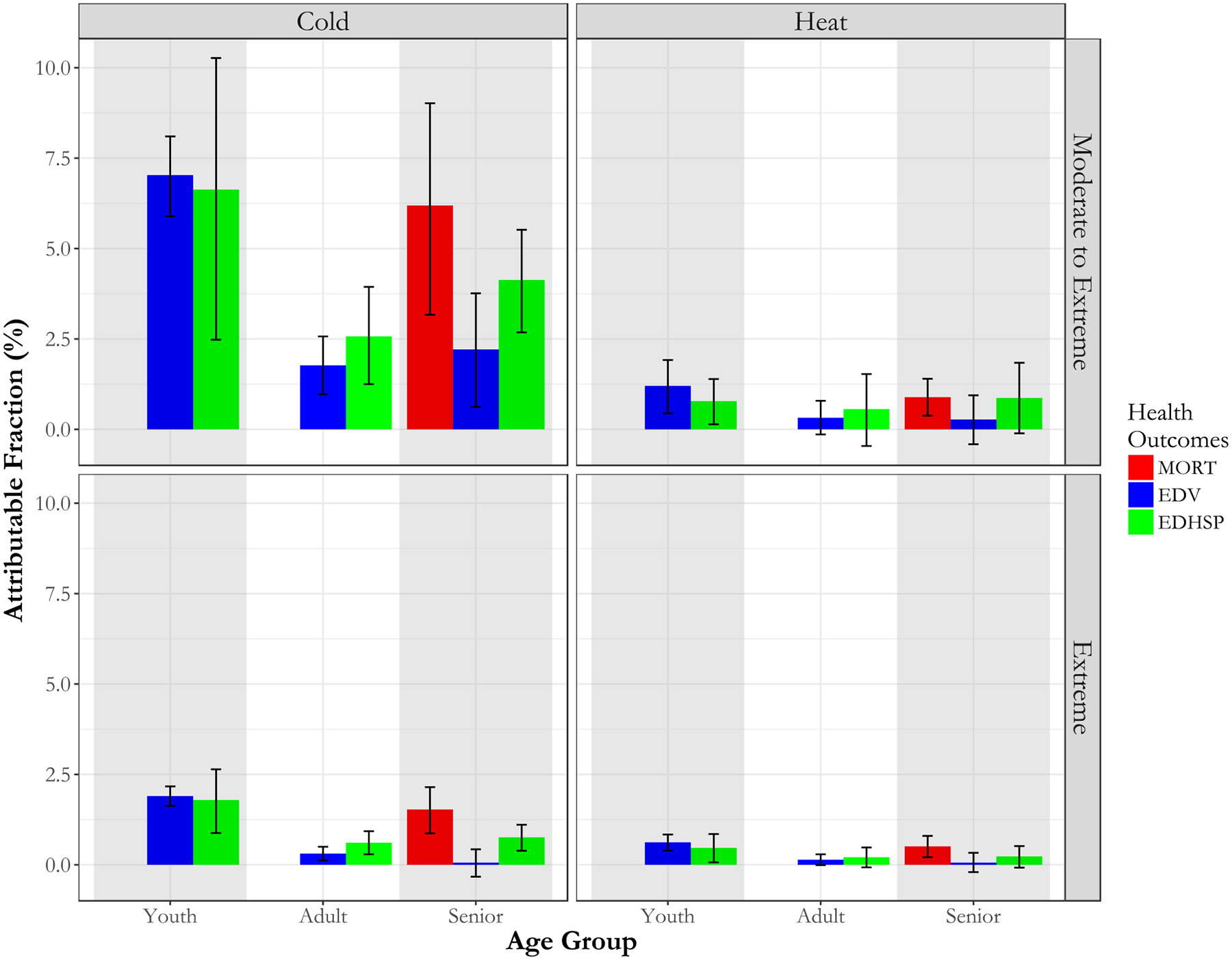
Attributable fraction of three health outcomes by age groups associated with temperature exposure. The uncertainty range is defined by 95% empirical confidence intervals obtained by Monte Carlo simulations (n = 5000). This figure does not include mortality results regarding 0–19 year olds or 20–64 year olds because there is no increased relative risk of mortality at any exposure level for these age groups.
Fig. 3.

Attributable cases of three health outcomes by age groups associated with temperature exposure. The uncertainty range is defined by 95% empirical confidence intervals obtained by Monte Carlo simulations (n = 5000). This figure does not include mortality results regarding 0–19 year olds or 20–64 year olds because there is no increased relative risk of mortality at any exposure level for these age groups.
We analyzed EDV and EDHSP results in the same way. Youth (0–19 years) is the only age group with a substantial health burden associated with heat exposures. There are 23,478 [95% eCI: 8751, 37,860] (1.2% [95% eCI: 0.4%, 1.9%]) cases of EDVs and 1089 [95% eCI: 194, 1929] (0.78% [95% eCI: 0.1%, 1.4%]) EDHSPs associated with moderate to extreme heat exposures. Among them, 12,079 [95% eCI: 7512, 16,420] (0.6% [95% eCI: 0.4%, 0.8%]) EDVs and 657 [95% eCI: 102, 1189] (0.5% [95% eCI: 0.1%, 0.9%]) EDHSPs are associated with extreme heat exposures. Heat exposures are not associated with health burden among adults (20–64 years) or seniors (65+ years) in the TCMA. Regarding cold, there are positive AFs and ACs for all health outcomes and for all age groups considering moderate to extreme exposures. Given EDV, youth has the highest AF as well as AC (7.03% [95% eCI: 5.9%, 8.1%], 137,622 [95% eCI: 115,749, 157,331], respectively). However, the EDHSP-specific analysis shows that although the youth has the highest AF (6.6% [95% eCI: 2.5%, 10.3%]), seniors have the highest AC (24,252 [95% eCI: 15,750, 32,327]). The underlying reason is that there are many more senior EDHSPs than youth EDHSPs. When we considered only extreme cold, all estimates become smaller, as expected, and the AF and AC among senior EDV cases were no longer positive; otherwise, all patterns were similar to those described above. The attributable EDHSPs for youth, adult, and senior are 2488 [95% eCI: 1225, 3680], 4372 [95% eCI: 1992, 6732], and 4445 [95% eCI: 2319, 6509] – their differences become smaller than that considering moderate to extreme cold exposures. Overall, youth is the most vulnerable but not always the most affected (measured by burden) age group. Based on EDHSP AC, seniors and adults are both have higher health burden compared to the youth. Numbers used to generate Figs. 2 and 3 are in Supplemental Information Section 6.
After taking into consideration inflation and income growth, based on total AC in the 65+ years age group and the VSL estimated by U.S. EPA (1997), the mortality costs related to moderate to extreme cold and heat exposures are $8119.33 million [95% eCI: $4158.15 million, $11,862.49million] and $1167.50 million [95% eCI: $478.11 million, $1839.77 million] per year, respectively. The mortality costs related to extreme cold and heat only are $2,00.67 million [95% eCI: $1152.52 million, $2809.77 million] and $665.06 million [95% eCI: $276.35, $1041.53 million] dollars per year, respectively. Using updated VSL values of Thomson and Monje (2015) did not lead to substantial changes in these estimates (Supplemental Information Section 4.1.5).
After taking into consideration inflation, the overall results show that the medical costs for EDHSP are higher than those of EDV due to the durations of stay. In addition, the medical costs due to cold exposures are higher than those of heat due to higher health burden (i.e. AC and AF). Among EDVs, the largest contributor to annual medical costs is the 0–19 years age group under cold exposure. This age group accounts for $8.18 million [95% eCI: $7.82 million, $8.54 million] in medical expenses associated with moderate to extreme cold exposures and $2.21 million [95% eCI: $2.11 million, $2.32 million] associated with only extreme cold exposures (Tables 2 and 3). Among EDHSPs, the largest contributor to annual medical costs is the 65+ year age group under cold exposure, which accounted for $37.20 million [95% eCI: $33.48 million, $40.85 million] in medical expenses associated with moderate to extreme cold exposures and $6.85 million [95% eCI: $5.81 million, $7.90 million] associated with only extreme cold exposures.
Table 2.
Cost estimates for each health outcomes by age groups (in million 2016 USD) attributable to moderate to extreme ambient temperature exposure.
| Health outcome | Cost criteria | Age group | Moderate-extreme cold exposure HI_max <30th percentile Expected value [95% eCI] |
Moderate-extreme heat exposure HI_max >70th percentile Expected value [95% eCI] |
|---|---|---|---|---|
| Mortality (MORT) | – | 0–19 | – | – |
| 20–64 | – | – | ||
| 65+ | 8119.33 [4158.15,11,862.49] |
1167.50 [478.11, 1839.77] |
||
| Emergency department visit (EDV) | Medical costs | 0–19 | 8.18 [7.82, 8.54] |
1.40 [1.15,1.65] |
| 20–64 | 7.17 [6.25, 8.11] |
– | ||
| 65+ | 2.54 [2.01, 3.06] |
– | ||
| Productivity loss | 0–19 | 0.16 [0.15, 0.16] |
0.03 [0.02, 0.03] |
|
| 20–64 | 1.64 [1.43,1.85] |
– | ||
| 65+ | 0.12 [0.10, 0.15] |
– | ||
| Emergency hospitalization (EDHSP) | Medical costs | 0–19 | 12.81 [10.63, 14.98] |
1.51 [1.11,1.94] |
| 20–64 | 27.69 [23.53,31.81] |
– | ||
| 65+ | 37.20 [33.48, 40.85] |
– | ||
| Productivity loss | 0–19 | 0.04 [0.03, 0.05] |
0.005 [0.004, 0.006] |
|
| 20–64 | 1.93 [1.63, 2.21] |
– | ||
| 65+ | 0.78 [0.71, 0.86] |
– | ||
| Total | – | – | 8215.18 [4908.92,11,357.45] |
1171.47 [614.26, 1749.07] |
Table 3.
Cost estimates for each health outcomes by age groups (in million 2016 USD) attributable to extreme ambient temperature exposure.
| Health outcome | Cost group | Age group | Extreme cold exposure HI_max <5th percentile (unit = $MM) Expected value [95% eCI] |
Extreme heat exposure HI_max >95th percentile (unit = $MM) Expected value [95% eCI] |
|---|---|---|---|---|
| Mortality (MORT) | – | 0–19 | – | – |
| 20–64 | – | – | ||
| 65+ | 2005.67 [1152.52, 2809.77] |
665.06 [276.35,1041.53] |
||
| Emergency department visit (EDV) | Medical costs | 0–19 | 2.21 [2.11,2.32] |
0.73 [0.65, 0.81] |
| 20–64 | 1.27 [1.00,1.54] |
– | ||
| 65+ | - | - | ||
| Productivity loss | 0–19 | 0.04 [0.04, 0.04] |
0.01 [0.01, 0.02] |
|
| 20–64 | 0.29 [0.23,0.35] |
– | ||
| 65+ | – | – | ||
| Emergency hospitalization (EDHSP) | Medical costs | 0–19 | 3.49 [2.87, 4.13] |
0.91 [0.63, 1.22] |
| 20–64 | 6.57 [5.39, 7.77] |
– | ||
| 65+ | 6.85 [5.81,7.90] |
– | ||
| Productivity loss | 0–19 | 0.01 [0.01,0.01] |
0.003 [0.002, 0.004] |
|
| 20–64 | 0.46 [0.38, 0.55] |
– | ||
| 65+ | 0.15 [0.12, 0.16] |
– | ||
| Total | – | – | 2033.24 [1318.64, 2725.38] |
667.61 [343.46, 993.11] |
Among adults (20–64 years), productivity loss was associated with relevant EDVs and EDHSPs under cold exposures. Considering moderate to extreme cold exposures among adults, the annual productivity loss is $1.63 million [95% eCI: $1.41 million, $1.84 million] due to EDVs and $1.93 million [95% eCI: $1.64 million, $2.22 million] due to EDHSPs. Considering extreme cold exposures only, the annual productivity loss is $0.29 million [95% eCI: $0.23 million, $0.35 million] due to EDVs and $0.46 million [95% eCI: $0.38 million, $0.55 million] due to EDHSPs.
Each year, the health burden associated with ambient temperature exposure leads to economic costs of approximately $9.40 billion [95% eCI: $6.05 billion, $12.57 billion] considering both moderate and extreme exposures and $2.70 billion [95% eCI: $1.91 billion, $3.48 billion] considering only extreme exposures in the TCMA. Morbidity loss makes up roughly 0.1–2.5% of the total costs depending exposure magnitude and age group.
4. Discussion
This study presents estimates of the health-related economic costs associated with ambient temperature exposures for the TCMA – approximately $9.40 billion annually when both extreme and moderate exposures are considered. This comprehensive estimate relies on multiple criteria, capturing different population health outcomes. The World Health Organization recommends the use of such multi-criteria approach for estimating health-related costs associated with climate change as a means of internalizing an array of external costs, enabling comparison across different outcomes, and providing explicit rules for balancing a range of information (Hutton et al., 2013). Based on such a multi-criteria approach, our results show that cold exposures are responsible for the economic costs for the TCMA considering mortality and emergency department visits. This holds true regardless of the health outcome or age group. Harsh winters and freezing temperatures pose serious health risks even for a well-acclimatized population. The methods developed in this study demonstrate strengths that recommend its application for other jurisdictions and types of environmental exposures.
Our findings highlight that temperature-related costs vary by age. Seniors are the only age group for which extreme temperature conditions are associated with increased mortality. These results are broadly consistent with Hajat et al. (2014), Dang et al. (2016), and Yang et al. (2012), which demonstrate that mortality associated with ambient temperature exposure is greater for persons 65 years or older compared to younger age groups. Consequently, the overall mortality costs are essentially mortality costs for seniors. Factors that make seniors more vulnerable to ambient temperature exposures include social isolation (Naughton et al., 2002), poverty (Basu and Ostro, 2008), a high prevalence of chronic health conditions (Hajat et al., 2014), and reduced ability to take preventive actions to mitigate exposures (Ebi et al., 2006). Regarding morbidity outcomes, the relative risks for youth increase more rapidly than other age groups as temperature move to the extremes of both cold and heat. Cold exposures affect all three age groups, consistent with the results of Cui et al. (2016) and Zhang et al. (2014). The youth age group has the highest AF associated with cold exposures. Heat exposures, on the other hand, affect only the youth. Regarding this particular observation, current literature provides inconsistent evidence (Nitschke et al., 2007, 2011; Kingsley et al., 2015; Zhang et al., 2014). It is important to keep in mind that there are many more senior EDHSP cases than youth cases. Seniors hospitalized after emergency department visits likely require more intensive and extensive medical services due to co-morbidities and reduced physiological capacity (Ebi et al., 2006; Hajat et al., 2014). Therefore, it is plausible that seniors contribute more to medical costs even though youth are associated with higher health risks of EDHSP given hazardous temperature exposure.
This study suggests that studies that limit to seniors a priori, under the assumption that other age groups are not as severely impacted by ambient temperatures, may be substantially underestimating the total health burden. There are a large number of individuals 0–19 years whose emergency department visits are also associated with ambient temperature although few of them result in death. Therefore, this study confirms that the youngest and the oldest age groups both need to be considered at risk (Sarofim et al., 2016; Xu et al., 2013). With regard to public health services, focusing on both the youngest and the oldest individuals appears necessary. This analysis provides information for supporting strategic prioritization of different age groups in intervention programs (e.g., risk communication and education). Specific application will depend on the objective of the decision maker. For instance, targeting youth is justifiable when the goal is to protect the most vulnerable individuals. Targeting seniors, especially when exposed to cold, may be more efficient in reducing the overall economic costs.
The multi-criteria developed in this study is an extension of the theoretical framework in Knowlton et al. (2011), with the goal of improving economic costs assessment of health risks associated with ambient temperature exposure. This design accounts for various different aspects of economic costs, such as medical expenses and productivity loss, simultaneous while considering a single mortality or morbidity case. The overall economic costs can be considered a composite indicator of impact measurement. This indicator allows for potential comparison between the public health consequences of different environmental exposures, such as air pollution and extreme temperature exposure, which involve multiple health outcomes and aspects of economic costs. The capacity for comparison is crucial to public health decision-makers with needs to prioritize at-risk population and allocate scarce resources to manage different environmental exposures.
Although different public health outcomes are eventually summed to obtain the total economic costs, it is easy to backtrack to the itemized cost criterion that contributes the most (or the least) to the overall economic burden. For instance, in our study, we attribute 98% of the total economic burden to mortality although the remaining 2% affects a much larger number of individuals (see Supplemental Information Section 7). The theoretical framework of this study is flexible. When new parameter estimates become available, cost estimates can be easily updated.
In the absence of personal exposure monitoring, the assignment of exposure(s) from sparsely spaced monitors to an entire population is imprecise. However, with this available exposure information, we attempt our best to establish an association of how temperature fluctuations affect adverse health outcomes and characterize this across a wide range of temperature extremes that could subsequently be used in public health messaging. There are some additional limitations. On mortality, we assume VSL to be insensitive to age. Although consistent with the current government practices (Thomson and Monje, 2015; U.S. EPA NCEE, 2010), this assumption’s validity, i.e. how VSL varies by age, is still up for debate among health economists (U.S. EPA NCEE, 2010) (Aldy and Viscusi, 2007). As for morbidity, we did not include non-emergent clinical visits due to data availability. Non-emergent morbidity could be potentially relevant to sub-optimal cold exposure, given the likely delayed effects (Anderson and Bell, 2009). Future studies should consider expanding to a more complete set of morbidity measures if data become available. This study considers only direct productivity losses. For instance, the DPV of those aged 0–14 years is 0 while calculating the overall DPV of the youth age-group (0–19 year olds). In other words, indirect losses such as time off work that was taken by parents who need to take care of their ill children are not included in the cost function, which may result in underestimation of the total real cost. Regarding the overall cost function, it is important to point out that by adding mortality costs and morbidity costs, theoretical costs (i.e., willingness-to-pay) are added to transactions that have actually occurred (i.e., medical bills). To compensate for this limitation, the itemized, as well as the overall costs of public health burden associated with hazardous ambient temperature exposures, are both provided.
5. Conclusion
This study estimates economic costs incurred by the health burden of ambient temperature exposures, a particularly relevant public health threat given the shifting temperature patterns due to climate change. The results can help develop effective public health interventions that target specific at-risk populations and inform resources allocation. Using multiple criteria to aggregate economic estimates across different age groups leads to a useful, transparent, and flexible composite indicator of costs. This approach can be adopted for assessing the overall impact of other environmental exposures, such as air pollution, that involve multiple health outcomes and aspects of costs.
Supplementary Material
HIGHLIGHTS.
The relationship between ambient temperature and population health varies by age group.
Suboptimal temperature is associated with serious mortality burden among elderly and morbidity burden among youth.
Suboptimal temperature is associated with large health-related economic costs in an urban setting.
Suboptimal low temperature has contributed more to health-related economic costs than suboptimal high temperature.
Acknowledgments
The authors appreciate the generous support from the National Weather Service (Chanhassen, Minnesota Forecast Office) and the Minnesota Pollution Control Agency in acquiring the necessary data.
Funding source
The research presented in this study is supported by the U.S. Centers for Disease Control and Prevention, Grant Number: 5H13EH001125-03.
Abbreviations
- CCR
Cost-to-charge ratio
- DPV
Daily production value
- DLNM
Distributed lag nonlinear model
- eCI
Empirical confidence interval
- EDHSP
Emergency department visits followed by hospitalization
- EDV
Emergency department visits followed by discharge
- EPA
Environmental Protection Agency
- HI
Heat index
- MDH
Minnesota Department of Health
- MET
Minimum effect temperature
- MM
Millions
- MORT
Mortality
- NWS
National Weather Service
- PFR
Professional-fee ratio
- RR
Relative risk
- TCMA
Minneapolis – St. Paul Twin Cities Metropolitan Area
- USD
U.S. dollar
- VSL
Value of a statistical life
Footnotes
Conflict of interests
The authors declare they have no actual or potential competing financial interests.
Disclaimer
The findings and conclusions in this report are those of the authors and do not necessarily represent the views of the Centers for Disease Control and Prevention.
Appendix A. Supplemental material
Supplementary data to this article can be found online at https://doi.org/10.1016/j.scitotenv.2019.04.398.
References
- Aldy JE, Viscusi WK, 2007. Age differences in the value of statistical life: revealed preference evidence. Rev. Environ. Econ. Policy 1 (2), 241–260. 10.1093/reep/rem014. [DOI] [Google Scholar]
- Analitis A, Katsouyanni K, Biggeri A, Baccini M, Forsberg B, Bisanti L, Michelozzi P, 2008. Effects of cold weather on mortality: results from 15 European cities within the PHEWE project. Am. J. Epidemiol 168 (12), 1397–1408. 10.1093/aje/kwn266. [DOI] [PubMed] [Google Scholar]
- Anderson BG, Bell ML, 2009. Weather-related mortality. Epidemiology 20 (2), 205–213. 10.1097/EDE.0b013e318190ee08. [DOI] [PMC free article] [PubMed] [Google Scholar]
- Basu R, 2009. High ambient temperature and mortality: a review of epidemiologic studies from 2001 to 2008. Environ. Health 8 (1), 40. 10.1186/1476-069X-8-40. [DOI] [PMC free article] [PubMed] [Google Scholar]
- Basu R, Ostro BD, 2008. A multicounty analysis identifying the populations vulnerable to mortality associated with high ambient temperature in California. Am. J. Epidemiol 168 (6), 632–637. 10.1093/aje/kwn170. [DOI] [PubMed] [Google Scholar]
- Berko J, Ingram DD, Saha S, Parker JD, 2014. Deaths attributed to heat, cold, and other weather events in the United States, 2006–2010. Natl. Health Stat. Rep 76, 1–15 Retrieved from. https://www.cdc.gov/nchs/data/nhsr/nhsr076.pdf. [PubMed] [Google Scholar]
- Chen H, Wang J, Li Q, Yagouti A, Lavigne E, Foty R, Copes R, 2016. Assessment of the effect of cold and hot temperatures on mortality in Ontario, Canada: a population-based study. CMAJ Open 4 (1), E48–E58. 10.9778/cmajo.20150111. [DOI] [PMC free article] [PubMed] [Google Scholar]
- The impacts of climate change on human health in the United States: a scientific assessment. In: Crimmins A, Balbus J, Gamble JL, Beard CB, Bell JE, Dodgen D (Eds.), U.S. Global Change Research Program, p. 312 Washington, DC. 10.7930/J0R49NQX. [DOI] [Google Scholar]
- Cui Y, Yin F, Deng Y, Volinn E, Chen F, Ji K, Li X, 2016. Heat or cold: which one exerts greater deleterious effects on health in a basin climate city? Impact of ambient temperature on mortality in Chengdu, China. Int. J. Environ. Res. Public Health 13 (12). 10.3390/ijerph13121225. [DOI] [PMC free article] [PubMed] [Google Scholar]
- Dang TN, Seposo XT, Duc NHC, Thang TB, An DD, Hang LTM, Honda Y, 2016. Characterizing the relationship between temperature and mortality in tropical and subtropical cities: a distributed lag non-linear model analysis in Hue, Viet Nam, 2009–2013. Glob. Health Action 9 (1). 10.3402/gha.v9.28738. [DOI] [PMC free article] [PubMed] [Google Scholar]
- Ebi KL, Mills DM, Smith JB, Grambsch A, 2006. Climate change and human health impacts in the United States: an update on the results of the U.S. National Assessment. Environ. Health Perspect 114 (9), 1318–1324. 10.1289/ehp.8880. [DOI] [PMC free article] [PubMed] [Google Scholar]
- Gasparrini A, Leone M, 2014. Attributable risk from distributed lag models. BMC Med. Res. Methodol 14, 55. 10.1186/1471-2288-14-55. [DOI] [PMC free article] [PubMed] [Google Scholar]
- Gasparrini A, Guo Y, Hashizume M, Lavigne E, Zanobetti A, Schwartz J, … Leone M, 2015. Mortality risk attributable to high and low ambient temperature: a multicountry observational study. The Lancet 386 (9991), 369–375. [DOI] [PMC free article] [PubMed] [Google Scholar]
- Gasparrini A, Guo Y, Hashizume M, Lavigne E, Tobias A, Zanobetti A, … Armstrong BG (2016). Changes in susceptibility to heat during summer: a multicountry analysis, 183(11), 18–20. doi: 10.1093/aje/kwv260. [DOI] [PMC free article] [PubMed] [Google Scholar]
- Gasparrinia A, Armstrong B, Kenward MG, 2010. Distributed lag non-linear models. Stat. Med 29 (21), 2224–2234. 10.1002/sim.3940. [DOI] [PMC free article] [PubMed] [Google Scholar]
- Graubard BI, Fears TR, 2005. Standard errors for attributable risk for simple and complex sample designs. Biometrics 61 (3), 847–855. 10.1111/j.1541-0420.2005.00355.x. [DOI] [PubMed] [Google Scholar]
- Grosse SD, Krueger KV, Mvundura M, 2009. Economic productivity by age and sex: 2007 estimates for the United States. Med. Care 47 (7 Suppl 1), S94–S103. 10.1097/MLR.0b013e31819c9571. [DOI] [PubMed] [Google Scholar]
- Hajat S, Vardoulakis S, Heaviside C, Eggen B, 2014. Climate change effects on human health: projections of temperature-related mortality for the UK during the 2020s, 2050s and 2080s. J. Epidemiol. Community Health, 1–8 10.1136/jech-2013-202449. [DOI] [PubMed] [Google Scholar]
- Hutton G, Menne B, 2014. Economic evidence on the health impacts of climate change in Europe. Environ. Health Insights, 43 10.4137/EHI.S16486. [DOI] [PMC free article] [PubMed] [Google Scholar]
- Hutton G, Sanchez G, Menne B, 2013. Climate Change and Health: A Tool to Estimate Health and Adaption Costs. Retrieved from. http://www.euro.who.int/__data/assets/pdf_file/0018/190404/WHO_Content_Climate_change_health_DruckII.pdf.
- Kenkel D, 2003. Using estimates of the value of a statistical life in evaluating consumer policy regulations. J. Consum. Policy 26 (1), 1–21. [Google Scholar]
- Kingsley SL, Eliot MN, Gold J, Vanderslice RR, Wellenius GA, 2015. Current and projected heat-related morbidity and mortality in Rhode Island. Environ. Health Perspect 460 (4), 1–8. 10.1289/ehp.1408826. [DOI] [PMC free article] [PubMed] [Google Scholar]
- Knowlton K, Rotkin-Ellman M, Geballe L, Max W, Solomon GM, 2011. Six climate change-related events in the United States accounted for about $14 billion in lost lives and health costs. Health Aff. 30 (11), 2167–2176. 10.1377/hlthaff.2011.0229. [DOI] [PubMed] [Google Scholar]
- Levit KR, Friedman B, Wong HS, 2013. Estimating inpatient hospital prices from state administrative data and hospital financial reports. Health Serv. Res 48 (5). 10.1111/1475-6773.12065 n/a–n/a. [DOI] [PMC free article] [PubMed] [Google Scholar]
- Lin S, Hsu WH, van Zutphen AR, Saha S, Luber G, Hwang SA, 2012. Excessive heat and respiratory hospitalizations in New York State: estimating current and future public health burden related to climate change. Environ. Health Perspect 120 (11), 1571–1577. 10.1289/ehp.1104728. [DOI] [PMC free article] [PubMed] [Google Scholar]
- Minnesota Department of Health, 2015. Minnesota Climate and Health Profile Report 2015. Minneapolis. Retrieved from. https://www.health.state.mn.us/communities/environment/climate/docs/mnprofile2015.pdf. [Google Scholar]
- Naughton MP, Henderson A, Mirabelli MC, Kaiser R, Wilhelm JL, Kieszak SM, … McGeehin MA (2002). Heat-related mortality during a 1999 heat wave in Chicago. Am. J. Prev. Med, 22(4), 221–227. doi: 10.1016/S0749-3797(02)00421-X. [DOI] [PubMed] [Google Scholar]
- Nitschke M, Tucker GR, Bi P, 2007. Morbidity and mortality during heatwaves in metropolitain Adelaide. Med. J. Aust 187 (11/12), 662–665. 10.1017/CBO9781107415324.004. [DOI] [PubMed] [Google Scholar]
- Nitschke M, Tucker GR, Hansen AL, Williams S, Zhang Y, Bi P, 2011. Impact of two recent extreme heat episodes on morbidity and mortality in Adelaide, South Australia: a case-series analysis. Environ. Health 10, 42. 10.1186/1476-069X-10-42. [DOI] [PMC free article] [PubMed] [Google Scholar]
- Peterson C, Xu L, Florence C, Grosse SD, Annest JL, 2015. Professional fee ratios for US hospital discharge data. Med. Care 53 (10), 840–849. 10.1097/MLR.0000000000000410 (Professional). [DOI] [PMC free article] [PubMed] [Google Scholar]
- Rothfusz LP, 1990. The heat index equation. National Weather Service Technical Attachment (SR 90–23) https://www.weather.gov/media/bgm/ta_htindx.PDF. [Google Scholar]
- Saha S, Brock JW, Vaidyanathan A, Easterling DR, Luber G, 2015. Spatial variation in hyperthermia emergency department visits among those with employer-based insurance in the United States – a case-crossover analysis. Environ. Health 14 (1), 20. 10.1186/s12940-015-0005-z. [DOI] [PMC free article] [PubMed] [Google Scholar]
- Sarofim MC, Saha S, Hawkins MD, Mills DM, Hess J, Horton RM, … St Juliana A, 2016. The impacts of climate change on human health in the United States: a scientific assessment. Global Climate Change Impacts in the United States, pp. 44–68 Washington, DC. 10.7930/J0MG7MDX. [DOI] [Google Scholar]
- Schmeltz MT, Petkova EP, Gamble JL, 2016. Economic burden of hospitalizations for heat-related illnesses in the United States, 2001–2010. Int. J. Environ. Res. Public Health 13 (9). 10.3390/ijerph13090894. [DOI] [PMC free article] [PubMed] [Google Scholar]
- Thomson K, Monje C, 2015. Guidance on Treatment of the Economic Value of a Statistical Life (VSL) in U.S. Department of Transportation Analyses - 2015 Adjustment Washington, DC. Retrieved from. https://cms.dot.gov/sites/dot.gov/files/docs/VSL2015_0.pdf. [Google Scholar]
- Tobías A, Armstrong B, Gasparrini A, 2017. Investigating uncertainty in the minimum mortality temperature: methods and application to 52 Spanish cities. Epidemiology 28 (1), 72–76. 10.1097/EDE.0000000000000567. [DOI] [PMC free article] [PubMed] [Google Scholar]
- U.S. Environmental Protection Agency, 2016. Climate Change Indicators in the United States, Ed. 4 https://www.epa.gov/sites/production/files/2016-08/documents/climate_indicators_2016.pdf.
- U.S. EPA, 1997. The benefits and costs of the Clean Air Act, 1970 to 1990. Retrieved from. https://www.epa.gov/sites/production/files/2015-06/documents/contsetc.pdf.
- U.S. EPA NCEE, 2010. Valuing Mortality Risk Reductions for Environmental Policy: A White Paper. p. 95.
- Xu Y, Dadvand P, Barrera-Gomez J, Sartini C, Mari-Dell’Olmo M, Borrell C, Basagana X, 2013. Differences on the effect of heat waves on mortality by sociodemographic and urban landscape characteristics. J. Epidemiol. Community Health 67 (6), 519–525. 10.1136/jech-2012-201899. [DOI] [PubMed] [Google Scholar]
- Yang J, Ou C-Q, Ding Y, Zhou Y-X, Chen P-Y, 2012. Daily temperature and mortality: a study of distributed lag non-linear effect and effect modification in Guangzhou. Environ. Health 11 (1), 63. 10.1186/1476-069X-11-63. [DOI] [PMC free article] [PubMed] [Google Scholar]
- Ye X, Wolff R, Yu W, Vaneckova P, Pan X, Tong S, 2011. Ambient temperature and morbidity: a review of epidemiological evidence. Environ. Health Perspect 120 (1), 19–28. 10.1289/ehp.1003198. [DOI] [PMC free article] [PubMed] [Google Scholar]
- Zhang Y, Yan C, Kan H, Cao J, Peng L, Xu J, Wang W, 2014. Effect of Ambient Temperature on Emergency Department Visits in Shanghai, China: A Time Series Study., pp. 1–8 10.1186/1476-069X-13-100. [DOI] [PMC free article] [PubMed] [Google Scholar]
Associated Data
This section collects any data citations, data availability statements, or supplementary materials included in this article.