In the comments of this X-post (and New Scientist article, [MS1]) it is pointed out that the counterexample found using Anthropic’s Fable 5 Large Language Model (LLM).
Remark: The points found in this notebook are different than those in the X-post .
Theory
In this section we provide a theoretical formulation of the Jacobian conjecture. For more a mathematically elaborated formulation see the Wikipedia article “Jacobian conjecture”, [Wk1].
Suppose and are polynomials of the variables and . Consider the 2-dimensional (2D) transformation (i.e., a vector valued function) . The Jacobian conjectures says that if the Jacobian determinant:
is a non-zero constant, then there must exist another pair of polynomials that invert transformation with the polynomials in and .
Below we show that the conjecture is not true using the 3D transformation polynomials proclaimed in this X post, [MS1].
Demonstration
In this section the Anthropic’s Fable 5 found counterexample is exemplified using corresponding definitions and invocations.
Definition of the counterexample polynomial mapping:
So, let us use a two-stage computation: we find first a solution with two different points, then we find a third point that is different that previously found two. Here is the two-point finding spec:
In this section we give a visual representation of the counterexample using a 3D contour plot — the found points are plotted in red. Here we derive a 3D contour plot of the polynomial transformation:
In[]:= AbsoluteTiming[
gr = ContourPlot3D[polyMap[x, y, z], {x, -c, c}, {y, -c, c}, {z, -c, c},
Contours -> 9,
ContourStyle -> Directive[Opacity[0.4]],
Mesh -> None,
PlotRange -> All
];
]
Out[]= {72.9755, Null}
Combine the 3D contour plot with the points found in the previous section (plotted in red):
This document (notebook) has a complete usage example of a thin Model Context Protocol (MCP) client of the Wolfram Language paclet “MCPClient”, [AAp1]. The MCP server is run in Docker — see “Docker MCP Toolkit”.
“MCPClient” provides a set of functions for using MCP server’s methods by converting them to LLMTool objects. Those objects can be used with Wolfram Language’s Large Language Model (LLM) framework.
Because the client is thin and its implementation concise, it is designed to allow both (i) quick, “on-the-spot” MCP utilization and (ii) easy understanding of MCP principles.
Remark: The Wolfram Language (WL) paclet “MCPClient”, [AAp1], has the same mission of the (Raku) package “MCP::Client”, [AAp2], but WL’s “MCPClient” uses a Functional Programming implementation instead of an Object-Oriented Programming one (as “MCP::Client” does.)
Remark: Note the distinction between an MCP-server (as, say, the one provided “AgentTools”, [WRIp1]) and an MCP-client. The former provides “tools”, the latter can interface with different (Docker, Python, WL, etc.) MCP servers.
Remark: The JSON file of MCP servers profile ingested and loaded in this section is an export of the manually made (default) profile using Docker’s dashboard.
MCP default profile in Docker’s dashboard:
Tools discovery and creation
Get the MCP server tools list:
mcpTools = MCPListTools[client, "Pause" -> 8];
Length[mcpTools]
Out[]= 75
Make a table of the tool records (only using names and descriptions) and show dimensions and a sample:
“Chatnik”, [AAp9], is a Wolfram Language (WL) paclet that provides Command Line Interface (CLI) scripts for conversing with multiple, persistent Large Language Model (LLM) personas. Files of the host Operating System (OS) are used to maintain persistence.
Most importantly, “Chatnik” does not try to entrench users in its own user experience (loop) for interaction with LLMs. Instead, it brings customizable LLM invocations and conversations into the Unix shell — making them composable, integratable, and scriptable with existing workflows.
In other words, the tag line “LLM Host in the Shell” should be understood as “LLMs, not as an app — but as a Unix shell primitive.”
Here are the most notable “Chatnik” features:
Provides UNIX shell pipelining for LLM interactions
Maintains a database of LLM chat objects
Connects to multiple models across different LLM providers
Offers access to a large repository of prompts
Enables convenient retrieval of interaction history
Includes management tools for the LLM chat object database
Preprocesses prompts using a simple domain-specific language (DSL)
Supports loading user-defined LLM personas from JSON files
Remark: “Chatnik” closely follows the LLM-chat objects interaction system of the Python package “JupyterChatbook”, [AAp3], and Raku package “Jupyter::Chatbook”, [AAp7]. Another (remote) resemblance can be found with the Wolfram Language paclet “Chatbook”, [CGp1]. (In other words, using OS shells instead of Jupyter or Wolfram notebooks.)
Remark: The WL paclet “Chatnik”, [AAp9], is a translation of the Raku package “Chatnik”, [AAp8] and the Python package “Chatnik”, [AAp4]. The WL CLI scripts are with CamelCase, i.e. LLMChat, LLMChatMeta, and LLMPrompt. The corresponding CLI scripts of the Raku package use kebab-case, i.e. llm-chat, llm-chat-meta, and llm-prompt. The corresponding CLI scripts of the Python package use snake_case, i.e. llm_chat, llm_chat_meta, and llm_prompt.
Remark: In addition, the Raku package provides the “umbrella” CLI chatnik.
Remark: When the phrase “Chatnik system” is used that is in order to emphasize that there are “Chatnik” packages in several programming languages with (almost) the same design and usage.
The rest of this document is organized as follows:
Introductory examples
Why make another LLM-CLI system?
Architectural design
Related and alternative packages
Introductory examples
The examples in this section demonstrate how the CLI scripts LLMChat and LLMChatMeta — provided by “Chatnik” — are used to have multi-turn LLM conversations and compose Unix shell pipelines with LLM interaction messages.
Remark: In order to use these scripts use the function ChatnikCopyScripts after installing “Chatnik”.
Remark: The prompts used in the examples are provided by the Wolfram Prompt Repository (WPR). Many of those prompts are also available in Python and Raku via the packages “LLMPrompts”, [AAp2], and “LLM::Prompts”, [AAp6], respectively.
Chat with Yoda
Here we create an LLM persona — by naming it and “priming it” with a prompt — and start interacting with it:
LLMChat 'Hi! Who are you?'--chat-id=yoda --prompt=@Yoda
# Yoda, I am. Wise and old Jedi Master, yes. Guide you, I can. Help, you seek?
Here we continue the conversation — using the --i synonym of --chat-id:
LLMChat 'How many students did you have?'--i=yoda
# Many students, I had. Countless, their lessons and destinies were. Luke Skywalker, among them, powerful Jedi he became. Teach, I did, those ready were. Hmm. Yes.
And continue the discussion some more:
LLMChat 'Which student is the best?'--i=yoda
# Best student, difficult to say it is. Each, unique journey they have. Luke Skywalker, strong in the Force he is. But compassion, patience, and wisdom, important they are. Judge by these, you must. Hmm. Yes.
The example used the LLM persona “Yoda”. (See more LLM personas here.)
Fortune-echo-limerick pipeline
Here we specify a pipeline for
Getting a fortune
Echoing it
Using the fortune to make a limerick
fortune | tee /dev/tty | LLMChat --prompt="Make a limerick from the given text:"
I have made this letter longer than usual because I lack the time to
make it shorter.
-- Blaise Pascal
There once was a note, quite verbose,
Longer than needed, I suppose.
Pascal said with a grin,
“To be short takes more spin,”
So brevity’s craft he chose to oppose.
Remark: In the shell command above, LLMChat created (or reused) a chat object with the default identifier “NONE”.
Since the result is given in Markdown code fences we take the last message via the CLI script LLMMetaChat, then use sed to remove the first and last lines, and then pass that text to the terminal Mermaid-JS visualizer mmdflux:
LLMChatMeta last-message --i=mmd | sed '1d; $d' | mmdflux
┌───────────────┐ ┌──────┐ ┌────────┐
│ Blaise Pascal │ │ Note │ │ Reader │
└───────┬───────┘ └───┬──┘ └────┬───┘
│ │ │
│─Write verbose letter──────────────>│ │
│ │ │
│ │─Deliver longer-than-usual message─>│
│ │ │
│─"To be short takes more spin"──────────────────────────────────────────>│
│ │ │
│ │─"Brevity's craft opposed"─────────>│
│ │ │
Remark: Since the result is usually given in Markdown code fences, we did not make a pipeline to plot the diagram. We used two shell commands in order to observe the intermediate result.
Remark: The default object identifier for both LLMChat and LLMChatMeta is “NONE”.
Copy-editing
Here is a very practical example — this document was copy-edited with the prompt “CopyEdit” using the following commands:
open Chatnik-LLM-Host-in-the-Shell-Part-1_edited.md
(And, yes, the LLM copy-edited version was evaluated, and some edits were rejected.)
Why make another LLM-CLI system?
Some questions to answer
Why do it?
Why was it relatively easy to do?
Why is it useful?
Why do it?
Most LLM interfaces — both “big” popular ones and those built by developers experimenting with LLMs — default to an application-centric design: a closed interaction loop with implicit state. This pattern is convenient, but very limiting. It can be cynically seen as an intentional effort for user lock-in or just as an attempt to impose certain user-experience views. It works against the “freedom enabling” Unix design principles. (Such as composability, transparency, and scriptability.)
With “Chatnik”, instead of adapting workflows to fit an LLM application, LLM capabilities are brought into the shell as first-class primitives. This enables reuse of existing tooling (pipes, redirects, scripts) and aligns LLM interaction with long-established UNIX practices.
Why was it relatively easy to do?
“Chatnik” is a composition of existing capabilities rather than a ground-up implementation:
Modern LLM providers (e.g., OpenAI, Google, Ollama) expose messy, non-uniform APIs that should be abstracted behind a single interface
The Raku ecosystem already provides flexible text processing, DSL making and usage, and CLI tooling
The “LLM::Functions” package encapsulates model interaction patterns, reducing knowledge of concrete APIs
Persistence can be implemented with simple file-based storage, avoiding the need for complex infrastructure
Remark: Related to the last point above, the following quote is attributed to Ken Thompson about UNIX:
We have persistent objects, they’re called files.
Remark: Less obnoxiously, instead of saying that LLM providers expose messy, non-uniform APIs, we can say that their APIs “are individually reasonable, but collectively inconsistent.” Because of the popularity of OpenAI’s models, many LLM providers adhere to a degree with OpenAI’s API. Still, the APIs — collectively — have inconsistent schemas, authorization, streaming, tool-calling, roles, etc.
Why is it useful?
“Chatnik” is useful because it places LLM capabilities in a natural manner into Unix shell workflows:
LLM calls can be embedded into shell pipelines, enabling automation and chaining
Conversations are persistent and inspectable via the file system
Prompt reuse and DSL preprocessing reduce repetition and keep workflows clear
Multiple providers can be used interchangeably without changing workflows
Existing UNIX tools (e.g., grep, awk, sed) can be combined with LLM outputs
Also, additional “widgets”, like Markdown viewers, Mermaid-JS renderers, etc.
Architectural design
The following flowchart summarizes the computational components and their interactions fairly well:
Here is a concise narration of the flow:
A chat command is issued from the OS shell, triggering ingestion of the chat objects file into an in-memory chat database.
If a chat ID is specified and exists, the corresponding chat object is retrieved; otherwise, a new chat object is created (with a default “NONE” ID if unspecified).
The input is then processed through prompt parsing using a DSL. If known prompts are detected, they are expanded via the prompt repository; otherwise, the raw input proceeds directly.
The resulting message is evaluated through “LLM::Functions”, which mediates interaction with external providers such as OpenAI (ChatGPT), Google (Gemini), and Ollama.
The evaluation produces a chat result returned to the shell, while the updated chat state is written back to the chat objects file, ensuring persistence.
Expanded narration
Chatnik is built around the principle that LLM interaction should behave like a native shell capability, not a siloed application. A command issued in the OS shell is treated as the entry point into a composable pipeline, where LLM calls can participate alongside standard UNIX tools.
State is externalized and file-backed, not hidden in process memory. Chat sessions are represented as chat objects that are ingested from and persisted to the file system. This makes conversations durable, inspectable, and naturally versionable using existing OS tools.
Chat identity is explicit but optional. When a chat ID is provided, the corresponding conversation is resumed; when absent or unknown, a new chat object is created. This allows both ad-hoc interactions and long-lived conversational contexts without friction.
Prompting is treated as a programmable layer. Inputs are not passed directly to models; they are first parsed through a lightweight DSL. Known prompts are expanded from a prompt repository, enabling reuse, parameterization, and standardization of interactions.
LLM invocation is abstracted but not obscured. Evaluation is delegated to “LLM::Functions”, which provides a uniform interface over multiple providers, including OpenAI (ChatGPT), Google (Gemini), and Ollama. This keeps provider choice flexible while preserving a consistent workflow.
The system is designed for composability and integration. Each stage—state ingestion, prompt processing, evaluation, and persistence—can be understood as part of a pipeline. This makes LLM interactions scriptable, chainable, and interoperable with existing command-line utilities.
Persistence is a first-class outcome of every interaction. Every evaluation both returns a result to the shell and updates the underlying chat object store, ensuring that conversational context evolves incrementally and reliably.
In short. To reiterate the point in the introduction, “Chatnik” treats LLMs as shell-native, stateful, and programmable primitives — aligning conversational AI with the philosophy of UNIX pipelines rather than application-bound interfaces.
Related functions and packages
In this section, we point to Raku packages that are both ingredients of, and alternatives to, “Chatnik”.
Main ingredients
The LLM-chat object functionalities (creation and interaction) are provided by the Wolfram Language functions LLMConfiguration, [WRIf1], LLMPrompt, [WRIf2], and LLMSynthesize, [WRIf3]. In addition, the expansion of the prompt DSL, [SW1], is done by the function ChatnikPromptExpand.
The CLI script LLMPrompt of “Chatnik” can be used to examine, retrieve, and concretize prompts. For example, here it can be seen the full text of the function prompt “MermaidDiagram” with given arguments:
LLMPrompt MermaidDiagram MYTEXT MY_DIAGRAM_TYPE
In some cases it is more convenient to use LLMPrompt than prompt expansion. For example:
LLMChat "FOCUS TEXT START :: $(cat README.md) :: FOCUS TEXT END" | LLMChat ---i=fb --prompt="$(LLMPrompt ThinkingHatsFeedback 'FOCUS TEXT')"
Here is the context (prompt) of the chat object “fb”:
LLMChatMeta context --i=fb
We can see the outcome of the LLMChat pipeline above with:
LLMChatMeta last-message --i=fb | cat > chat.md
The paclet “CommandLineParser”, [MSp1], is used to parse the CLI arguments of the “Chatnik” scripts. The parser has certain limitations:
The non-named CLI arguments must be placed before the named ones.
The named arguments allways start with --. (I.e. -i does not work, --i does.)
Happy Pi Day! Today (3/14) we celebrate the most famous mathematical constant: 𝞹 ≈ 3.141592653589793…
𝞹 is irrational and transcendental, appears in circles, waves, probability, physics, and random walks.
Wolfram Language (with its built-in 𝞹 constant, excellent rational support, symbolic programming, and vast collection of Number Theory functions) makes experimenting with 𝞹 especially easy and enjoyable.
In this document (notebook) we explore a selection of formulas and algorithms.
1. Continued fraction approximation
The built-in Wolfram Language (WL) constant Pi (or π ) can be computed to an arbitrary high precision:
Let us compare it with a continued fraction approximation. For example, using the (first) sequence line of On-line Encyclopedia of Integer Sequences (OEIS) A001203 produces π with precision 100:
Next, we show the Pareto principle manifestation of for the continued fraction terms. First we observe that the terms a distribution similar to Benford’s law :
This document (notebook) describes three ways of making mazes (or labyrinths) using graphs. The first two are based on rectangular grids; the third on a hexagonal grid.
All computational graph features discussed here are provided by the Graph functionalities of Wolfram Language.
TL;DR
Just see the maze pictures below. (And try to solve the mazes.)
Procedure outline
The first maze is made by a simple procedure which is actually some sort of cheating:
A regular rectangular grid graph is generated with random weights associated with its edges.
The (minimum) spanning tree for that graph is found.
That tree is plotted with exaggeratedly large vertices and edges, so the graph plot looks like a maze.
This is “the cheat” — the maze walls are not given by the graph.
The second maze is made “properly”:
Two interlacing regular rectangular grid graphs are created.
The second one has one less row and one less column than the first.
The vertex coordinates of the second graph are at the centers of the rectangles of the first graph.
The first graph provides the maze walls; the second graph is used to make paths through the maze.
In other words, to create a solvable maze.
Again, random weights are assigned to edges of the second graph, and a minimum spanning tree is found.
There is a convenient formula that allows using the spanning tree edges to remove edges from the first graph.
In that way, a proper maze is derived.
The third maze is again made “properly” using the procedure above with two modifications:
Two interlacing regular grid graphs are created: one over a hexagonal grid, the other over a triangular grid.
The hexagonal grid graph provides the maze walls; the triangular grid graph provides the maze paths.
Since the formula for wall removal is hard to derive, a more robust and universal method based on nearest neighbors is used.
Simple Maze
In this section, we create a simple, “cheating” maze.
Remark: The steps are easy to follow, given the procedure outlined in the introduction.
The “maze” above looks like a maze because the vertices and edges are rectangular with matching sizes, and they are thicker than the spaces between them. In other words, we are cheating.
To make that cheating construction clearer, let us plot the shortest path from the bottom left to the top right and color the edges in pink (salmon) and the vertices in red:
finder = Nearest[Thread[GraphEmbedding[g1] -> VertexList[g1]]]
Take a maze edge and its vertex points:
e = First@EdgeList[mazePath];
aMazePathCoords = Association@Thread[VertexList[mazePath] -> GraphEmbedding[mazePath]];
 points = List @@ (e /. aMazePathCoords)
Find the edge’s midpoint and the nearest wall-graph vertices:
This document (notebook) discusses number theory properties and relationships of the integer 2026.
The integer 2026 is semiprime and a happy number, with 365 as one of its primitive roots. Although 2026 may not be particularly noteworthy in number theory, this provides a great excuse to create various elaborate visualizations that reveal some interesting aspects of the number.
A happy number is a number for which iteratively summing the squares of its digits eventually reaches 1 (e.g., 13 -> 10 -> 1). Here is a check that 2026 is happy:
ResourceFunction["HappyNumberQ"][2026]
Out[]= True
Here is the corresponding trail of digit-square sums:
The decomposition of $2026$ as $2 * 1013$ means the multiplicative group modulo $2026$ has primitive roots. A primitive root exists for an integer $n$ if and only if $n$ is $1$, $2$,$4$, $p^k$ , or $2 p^k$ , where $k$ is an odd prime and $k>0$ .
We can check additional facts about 2026, such as whether it is “square-free” , among other properties. However, let us compare these with the feature-rich 2025 in the next section.
Comparison with 2025
Here is a side-by-side comparison of key number theory properties for 2025 and 2026.
Property
2025
2026
Notes
Prime or Composite
Composite
Composite
Both non-prime.
Prime Factorization
3^4 * 5^2 (81 * 25)
2 * 1013
2025 has repeated small primes; 2026 is a semiprime (product of two distinct primes).
Number of Divisors
15 (highly composite for its size)
4 (1, 2, 1013, 2026)
2025 has many divisors; 2026 has very few.
Perfect Square
Yes (45^2 = 2025)
No
Major highlight for 2025—rare square year.
Sum of Cubes
Yes (1^3 + 2^3 + … + 9^3 = (1 + … + 9)^2 = 2025)
No
Iconic property for 2025 (Nicomachus’s theorem).
Happy Number
No (process leads to cycle including 4)
Yes (repeated squared digit sums reach 1)
Key point for 2026—its main “happy” trait.
Harshad Number
Yes (divisible by 9)
No (not divisible by 10)
2025 qualifies; 2026 does not.
Primitive Roots
No
Yes
This is a relatively rare property to have.
Other Notable Traits
{(20 + 25)^2 = 2025, Sum of first 45 odd numbers, Deficient number, Many pattern-based representations}
{Even number, Deficient number, Few special patterns}
2025 is packed with elegant properties; 2026 is more “plain” beyond being happy.
Overall “Interest” Level
Highly interesting—celebrated in math communities for squares, cubes, and patterns
Relatively uninteresting—basic semiprime with no standout geometric or sum properties
Reinforces blog’s angle.
To summarize:
2025 stands out as a mathematically rich number, often highlighted in puzzles and articles for its perfect square status and connections to sums of cubes and odd numbers.
2026 , in contrast, has fewer flashy properties — it’s a straightforward even semiprime — but it qualifies as a happy number and it has a primitive root.
Here is a computationally generated comparison table of most of the properties found in the table above:
Let us create and plot a graph showing the trails of all happy numbers less than or equal to 2026. Below, we identify these numbers and their corresponding trails:
There is a theorem by Gauss stating that any integer can be represented as a sum of at most three triangular numbers. Here we find an “interesting” solution:
sol = FindInstance[{2026 == PolygonalNumber[i] + PolygonalNumber[j] + PolygonalNumber[k], i > 10, j > 10, k > 10}, {i, j, k}, Integers]
Remark: It is interesting that 365 (the number of days in a common calendar year) is a primitive root of the multiplicative group generated by 2026 . Not many years have this property this century; many do not have primitive roots at all.
Here we find the position of 2026 in that sequence:
Position[seq, 2026]
Out[]= {{18}}
Given the title of the sequence and the extracted position of $2026$ , this means that the number of disconnected 4-regular graphs with 17 vertices is $2026$. ($17$ because the sequence offset is $0$.) Let us create a few graphs from that set by using the 5-vertex complete graph $\left(K_5\right.$) and circulant graphs . Here is an example of such a graph:
Number theory provides many opportunities for visualizations, so I included utilities for some of the popular patterns in “Math::NumberTheory”, [AAp1] and “NumberTheoryUtilities”.
The number of years in this century that have primitive roots and have 365 as a primitive root is less than the number of years that are happy numbers.
I would say I spent too much time finding a good, suitable, Christmas-themed combination of colors for the trails graph.
This document (notebook) discusses different combinations of Grammar-Based Parser-Interpreters (GBPI) and Large Language Models (LLMs) to generate executable code from Natural Language Computational Specifications (NLCM). We have the soft assumption that the NLCS adhere to a certain relatively small Domain Specific Language (DSL) or use terminology from that DSL. Another assumption is that the target software packages are not necessarily well-known by the LLMs, i.e. direct LLM requests for code using them would produce meaningless results.
We want to do such combinations because:
GBPI are fast, precise, but with a narrow DSL scope
LLMs can be unreliable and slow, but with a wide DSL scope
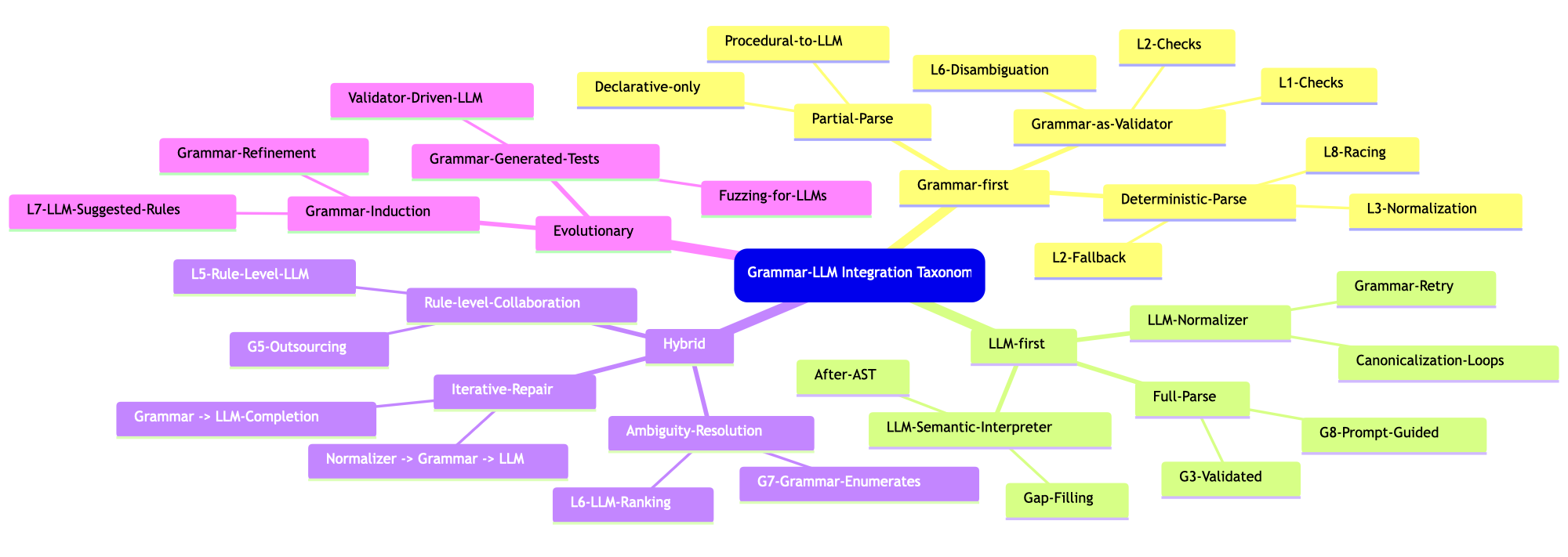
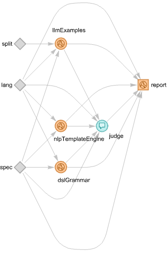
Because of GBPI and LLMs are complementary technologies with similar and overlapping goals the possible combinations are many. We concentrate on two of the most straightforward designs: (1) judged parallel race of methods execution, and (2) using LLMs as a fallback method if grammar parsing fails. We show asynchronous programmingimplementations for both designs using the Wolfram Language function LLMGraph.
The rest of the document is structured as follows:
Initial grammar-LLM combinations
Assumptions, straightforward designs, and trade-offs
Comprehensive combinations enumeration (attempt)
Tabular and morphological analysis breakdown
Three methods for parsing ML DSL specs into Raku code
One grammar-based, two LLM-based
Parallel execution with an LLM judge
Straightforward, but computationally wasteful and expensive
Grammar-to-LLM fallback mechanism
The easiest and most robust solution
Concluding comments and observations
TL;DR
Combining grammars and LLMs produces robust translators.
Three translators with different faithfulness and coverage are demonstrated and used.
Two of the simplest, yet effective, combinations are implemented and demonstrated.
Parallel race and grammar-to-LLM fallback.
Asynchronous implementations with LLM-graphs are a very good fit!
Just look at the LLM-graph plots (and be done reading.)
Initial Combinations and Associated Assumptions
The goal is to combine grammar-based parser-interpreters with LLMs in order to achieve robust parsing and interpretation of computational workflow specifications.
Here are some example combinations of these approaches:
A few methods, both grammar-based and LLM-based, are initiated in parallel. Whichever method produces a correct result first is selected as the answer.
This approach assumes that when the grammar-based methods are effective, they will finish more quickly than the LLM-based methods.
The grammar method is invoked first; if it fails, an LLM method (or a sequence of LLM methods) is employed.
LLMs are utilized at the grammar-rule level to provide matching objects that the grammar can work with.
If the grammar method fails, an LLM normalizer for user commands is invoked to generate specifications that the grammar can parse.
It is important to distinguish between declarative specifications and those that prescribe specific steps.
For a workflow given as a list of steps the grammar parser may successfully parse most steps, but LLMs may be required for a few exceptions.
The main trade-off in these approaches is as follows:
Grammar methods are challenging to develop but can be very fast and precise.
Precision can be guaranteed and rigorously tested.
LLM methods are quicker to develop but tend to be slower and can be unreliable, particularly for less popular workflows, programming languages, and packages.
Also, combinations based on LLM tools (aka LLM external function calling) are not considered because LLM-tools invocation is too unpredictable and unreliable.
Comprehensive breakdown (attempt)
This section has a “concise” table that expands the combinations list above into the main combinatorial strategies for Grammar *** LLMs** for robust parsing and interpretation of workflow specifications. The table is not an exhaustive list of such combinations, but illustrates their diversity and, hopefully, can give ideas for future developments.
A few summary points (for table’s content/subject):
The most robust systems combine grammar precision with LLM adaptability , typically by putting grammars first and using LLMs for repair, normalization, expansions, or semantic interpretation (i.e. “fallback”.)
Table: Combination Patterns for Parsing Workflow Specifications
tbl = Dataset[{<|"ID" -> 1, "CombinationPattern" -> "Parallel Race: Grammar + LLM", "Description" -> "Launch grammar-based parsing and one or more LLM interpreters in parallel; whichever yields a valid parse first is accepted.", "Pros" -> {"Fast when grammar succeeds", "Robust fallback", "Reduces latency unpredictability of LLMs"}, "ConsTradeoffs" -> {"Requires orchestration", "Need a validator for LLM output"}|>, <|"ID" -> 2, "CombinationPattern" -> "Grammar-First, LLM-Fallback", "Description" -> "Try grammar parser first; if it fails, invoke LLM-based parsing or normalization.", "Pros" -> {"Deterministic preference for grammar", "Testable correctness when grammar succeeds"}, "ConsTradeoffs" -> {"LLM fallback may produce inconsistent structures"}|>, <|"ID" -> 3, "CombinationPattern" -> "LLM-Assisted Grammar (Rule-Level)", "Description" -> "Individual grammar rules delegate to an LLM for ambiguous or context-heavy matching; LLM supplies tokens or AST fragments.", "Pros" -> {"Handles complexity without inflating grammar", "Modular LLM usage"}, "ConsTradeoffs" -> {"LLM behavior may break rule determinism", "Harder to reproduce"}|>, <|"ID" -> 4, "CombinationPattern" -> "LLM Normalizer -> Grammar Parser", "Description" -> "When grammar fails, LLM rewrites/normalizes input into a canonical form; grammar is applied again.", "Pros" -> {"Grammar remains simple", "Leverages LLM skill at paraphrasing"}, "ConsTradeoffs" -> {"Quality depends on normalizer", "Feedback loops possible"}|>, <|"ID" -> 5, "CombinationPattern" -> "Hybrid Declarative vs Procedural Parsing", "Description" -> "Grammar extracts structural/declarative parts; LLM interprets procedural/stepwise parts or vice versa.", "Pros" -> {"Each subsystem tackles what it's best at", "Reduces grammar complexity"}, "ConsTradeoffs" -> {"Harder to maintain global consistency", "Requires AST stitching logic"}|>, <|"ID" -> 6, "CombinationPattern" -> "Grammar-Generated Tests for LLM", "Description" -> "Grammar used to generate examples and counterexamples; LLM outputs are validated against grammar constraints.", "Pros" -> {"Powerful for verifying LLM outputs", "Reduces hallucinations"}, "ConsTradeoffs" -> {"Grammar must encode constraints richly", "Validation pipeline required"}|>, <|"ID" -> 7, "CombinationPattern" -> "LLM as Adaptive Heuristic for Grammar Ambiguities", "Description" -> "When grammar yields multiple parses, LLM chooses or ranks the \"most plausible\" AST.", "Pros" -> {"Improves disambiguation", "Good for underspecified workflows"}, "ConsTradeoffs" -> {"LLM can pick syntactically impossible interpretations"}|>, <|"ID" -> 8, "CombinationPattern" -> "LLM as Semantic Phase After Grammar", "Description" -> "Grammar creates an AST; LLM interprets semantics, fills in missing steps, or resolves vague ops.", "Pros" -> {"Clean separation of syntax vs semantics", "Grammar ensures correctness"}, "ConsTradeoffs" -> {"Semantic interpretation may drift from syntax"}|>, <|"ID" -> 9, "CombinationPattern" -> "Self-Healing Parse Loop", "Description" -> "Grammar fails -> LLM proposes corrections -> grammar retries -> if still failing, LLM creates full AST.","Pros" -> {"Iterative and robust", "Captures user intent progressively"}, "ConsTradeoffs" -> {"More expensive; risk of oscillation"}|>, <|"ID" -> 10, "CombinationPattern" -> "Grammar Embedding Inside Prompt Templates", "Description" -> "Grammar definitions serialized into the prompt, guiding the LLM to conform to the grammar (soft constraints).", "Pros" -> {"Faster than grammar execution in some cases", "Encourages consistent structure"}, "ConsTradeoffs" -> {"Weak guarantees", "LLM may ignore grammar"}|>, <|"ID" -> 11, "CombinationPattern" -> "LLM-Driven Grammar Induction or Refinement", "Description" -> "LLM suggests new grammar rules or transformations; developer approves; the grammar evolves over time.", "Pros" -> {"Faster grammar evolution", "Useful for new workflow languages"}, "ConsTradeoffs" -> {"Requires human QA", "Risk of regressing accuracy"}|>, <|"ID" -> 12, "CombinationPattern" -> "Regex Engine as LLM Guardrail", "Description" -> "Regex or token rules used to validate or filter LLM results before accepting them.", "Pros" -> {"Lightweight constraints", "Useful for quick prototyping"}, "ConsTradeoffs" -> {"Regex too weak for complex syntax"}|>}];

 tbl = tbl[All, KeyDrop[#, "ID"] &];
 tbl = tbl[All, ReplacePart[#, "Pros" -> ColumnForm[#Pros]] &];
 tbl = tbl[All, ReplacePart[#, "ConsTradeoffs" -> ColumnForm[#ConsTradeoffs]] &];
 tbl = tbl[All, Style[#, FontFamily -> "Times New Roman"] & /@ # &];
 ResourceFunction["GridTableForm"][tbl]
#
CombinationPattern
Description
Pros
ConsTradeoffs
1
Parallel Race: Grammar + LLM
Launch grammar-based parsing and one or more LLM interpreters in parallel; whichever yields a valid parse first is accepted.
{{Fast when grammar succeeds}, {Robust fallback}, {Reduces latency unpredictability of LLMs}}
{{Requires orchestration}, {Need a validator for LLM output}}
2
Grammar-First, LLM-Fallback
Try grammar parser first; if it fails, invoke LLM-based parsing or normalization.
{{Deterministic preference for grammar}, {Testable correctness when grammar succeeds}}
{{LLM fallback may produce inconsistent structures}}
3
LLM-Assisted Grammar (Rule-Level)
Individual grammar rules delegate to an LLM for ambiguous or context-heavy matching; LLM supplies tokens or AST fragments.
{{Handles complexity without inflating grammar}, {Modular LLM usage}}
{{LLM behavior may break rule determinism}, {Harder to reproduce}}
4
LLM Normalizer -> Grammar Parser
When grammar fails, LLM rewrites/normalizes input into a canonical form; grammar is applied again.
{{Grammar remains simple}, {Leverages LLM skill at paraphrasing}}
{{Quality depends on normalizer}, {Feedback loops possible}}
5
Hybrid Declarative vs Procedural Parsing
Grammar extracts structural/declarative parts; LLM interprets procedural/stepwise parts or vice versa.
{{Each subsystem tackles what it’s best at}, {Reduces grammar complexity}}
{{Harder to maintain global consistency}, {Requires AST stitching logic}}
6
Grammar-Generated Tests for LLM
Grammar used to generate examples and counterexamples; LLM outputs are validated against grammar constraints.
{{Powerful for verifying LLM outputs}, {Reduces hallucinations}}
{{Grammar must encode constraints richly}, {Validation pipeline required}}
7
LLM as Adaptive Heuristic for Grammar Ambiguities
When grammar yields multiple parses, LLM chooses or ranks the “most plausible” AST.
{{Improves disambiguation}, {Good for underspecified workflows}}
{{LLM can pick syntactically impossible interpretations}}
8
LLM as Semantic Phase After Grammar
Grammar creates an AST; LLM interprets semantics, fills in missing steps, or resolves vague ops.
{{Clean separation of syntax vs semantics}, {Grammar ensures correctness}}
{{Semantic interpretation may drift from syntax}}
9
Self-Healing Parse Loop
Grammar fails -> LLM proposes corrections -> grammar retries -> if still failing, LLM creates full AST.
{{Iterative and robust}, {Captures user intent progressively}}
{{More expensive; risk of oscillation}}
10
Grammar Embedding Inside Prompt Templates
Grammar definitions serialized into the prompt, guiding the LLM to conform to the grammar (soft constraints).
{{Faster than grammar execution in some cases}, {Encourages consistent structure}}
{{Weak guarantees}, {LLM may ignore grammar}}
11
LLM-Driven Grammar Induction or Refinement
LLM suggests new grammar rules or transformations; developer approves; the grammar evolves over time.
{{Faster grammar evolution}, {Useful for new workflow languages}}
{{Requires human QA}, {Risk of regressing accuracy}}
12
Regex Engine as LLM Guardrail
Regex or token rules used to validate or filter LLM results before accepting them.
{{Lightweight constraints}, {Useful for quick prototyping}}
{{Regex too weak for complex syntax}}
Diversity reasons
The diversity of combinations in the table above arises because Raku grammars and LLMs occupy fundamentally different but highly complementary positions in the parsing spectrum.
Raku grammars provide determinism, speed, verifiability, and structural guarantees, but they require upfront design and struggle with ambiguity, informal input, and evolving specifications.
LLMs, in contrast, excel at normalization, semantic interpretation, ambiguity resolution, and adapting to fluid or poorly defined languages, yet they lack determinism, may hallucinate, and are slower.
When these two technologies meet, every architectural choice — who handles syntax, who handles semantics, who runs first, who validates whom, who repairs or refines — defines a distinct strategy.
Hence, the design space naturally expands into many valid hybrid patterns rather than a single “best” pipeline.
That said, the fallback pattern implemented below can be considered the “best option” from certain development perspectives because it is simple, effective, and has fast execution times.
This section demonstrates the use of three different translation methods:
Grammar-based parser-interpreter of computational workflows
LLM-based translator using few-shot learning with relevant DSL examples
Natural Language Processing (NLP) interpreter using code templates and LLMs to fill-in the corresponding parameters
The translators are ordered according of their faithfulness, most faithful first. It can be said that at the same time, the translators are ordered according to their coverage — widest coverage is by the last.
Grammar-based
Here a recommender pipeline specified with natural language commands is translated into Raku code of the package “ML::SparseMatrixRecommender” using a sub of the paclet “DSLTranslation”:
spec = "create from dsData; apply LSI functions IDF, None, Cosine; recommend by profile for passengerSex:male, and passengerClass:1st; join across using dsData; echo the pipeline value";
The function DSLTranslation uses a web service by default but if Raku and the package “DSL::Translators” are installed it can use the provided Command Line Interface (CLI):
LLM translations can be done using a set of from-to rules. This is the so-called few shot learning of LLMs. The paclet “DSLExamples” has a collection of such examples for different computational workflows. (Mostly ML at this point.) The examples are hierarchically organized by programming language and workflow name; see the resource file “dsl-examples.json”, or execute DSLExamples[].
Here is a table that shows the known DSL translation examples in “DSL::Examples” :
Here is a recommender pipeline specified with natural language commands:
spec = "new recommender; create from @dsData; apply LSI functions IDF, None, Cosine; recommend by profile for passengerSex:male, and passengerClass:1st; join across with @dsData on \"id\"; echo the pipeline value; classify by profile passengerSex:female, and passengerClass:1st on the tag passengerSurvival; echo value";
commands = StringSplit[spec, ""];
Translate to WL code line-by-line:
res = LLMPipelineSegment[] /@ commands; res = Map[StringTrim@StringReplace[#, RegularExpression["Output\h*:"] -> ""] &, res];
 res = StringRiffle[res, "==>"]
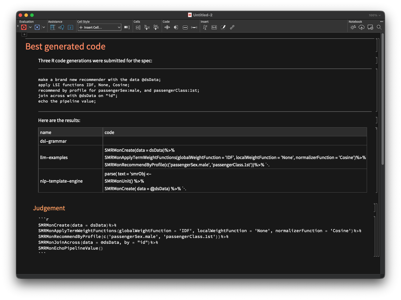
tmplJudge = StringTemplate["Choose the generated code that most fully adheres to the spec:\\n\\n\\n`spec`\\n\\n\\nfrom the following `lang` generation results:\\n\\n\\n1) DSL-grammar:\\n`dslGrammar`\\n\\n\\n2) LLM-examples:\\n`llmExamples`\\n\\n\\n3) NLP-template-engine:\\n`nlpTemplateEngine`\\n\\n\\nand copy it:"]
spec = " make a brand new recommender with the data @dsData; apply LSI functions IDF, None, Cosine; recommend by profile for passengerSex:male, and passengerClass:1st; join across with @dsData on \"id\"; echo the pipeline value; ";
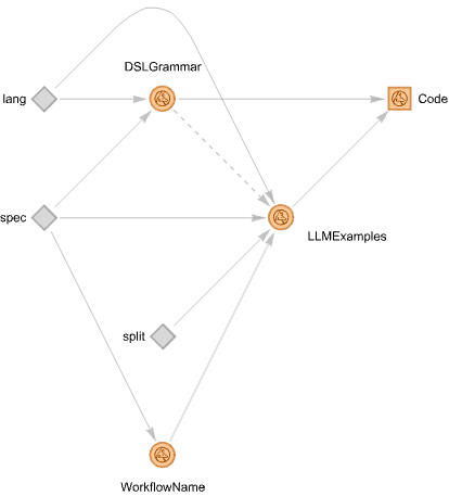
Instead of having DSL-grammar- and LLM computations running in parallel, we can make an LLM-graph in which the LLM computations are invoked if the DSL-grammar parsing-and-interpretation fails. In this section we make such a graph.
Before making the graph let us also generalize it to work with other ML workflows, not just recommendations.
Let us make an LLM function with a similar functionality. I.e. an LLM-function that classifies a natural language computation specification into workflow labels used by “DSLExamples”. Here is such a function using the sub LLMClassify provided by “NLPTemplateEngine”:
Here the LLM graph is run over a spec that can be parsed by DSL-grammar (notice the very short computation time):
Here is the obtained result:
Here is a spec that cannot be parsed by the DSL-grammar interpreter — note that there is just a small language change in the first line:
spec = " create from @dsData; apply LSI functions IDF, None, Cosine; recommend by profile for passengerSex:male, and passengerClass:1st; join across with @dsData on \"id\"; echo the pipeline value; ";
Nevertheless, we obtain a correct result via LLM-examples:
Let us specify another workflow — for ML-classification with Wolfram Language — and run the graph:
spec = " use the dataset @dsData; split the data into training and testing parts with 0.8 ratio; make a nearest neighbors classifier; show classifier accuracy, precision, and recall; echo the pipeline value; ";
Using LLM graphs gives the ability to impose desired orchestration and collaboration between deterministic programs and LLMs.
By contrast, the “inversion of control” of LLM – tools is “capricious.”
LLM-graphs are both a generalization of LLM-tools, and a lower level infrastructural functionality than LLM-tools.
The LLM-graph for the parallel-race translation is very similar to the LLM-graph for comprehensive document summarization described in [AA4].
The expectation that DSL examples would provide both fast and faithful results is mostly confirmed in ≈20 experiments.
Using the NLP template engine is also fast because LLMs are harnessed through QAS.
The DSL examples translation had to be completed with a workflow classifier.
Such classifiers are also part of the implementations of the other two approaches .
The grammar – based one uses a deterministic classifier, [AA1]
The NLP template engine uses an LLM classifier .
An interesting extension of the current work is to have a grammar-LLM combination in which when the grammar fails then the LLM “normalizes” the specs until the grammar can parse them.
Currently, LLMGraph does not support graphs with cycles, hence this approach “can wait” (or be implemented by other means .)
Multiple DSL examples can be efficiently derived by random sentence generation with different grammars.
Similar to the DSL commands classifier making approach taken in [AA1] .
LLMs can be also used to improve and extend the DSL grammars.
And it is interesting to consider automating that process, instead of doing it via human supervision.
Program a few versions of circle chords based visualization routines.
Called chord trail plots below.
Marvel at chord trail plots for larger moduli.
Make multiple collections of them.
Look into number of primitive roots distributions.
Consider making animations of the collections.
The animations should not be “chaotic” — they should have some inherent visual flow in them.
Consider different ways of sorting chord trail plots.
Using number theoretic arguments.
Yeah, would be nice, but requires too much head scratching and LLM-ing.
Convert plots to images and sort them.
Some might say that that is a “brute force” application.
Simple image sort does not work.
Latent Semantic Analysis (LSA) application.
After failing to sort the chord trail image collections by “simple” means, the idea applying LSA came to mind.
LSA being, of course, a favorite technique that was applied to sorting images multiple times in the past, in different contexts, [AAn1, AAn3, AAn4, AAn5, AAv3].
The function ChordTrails can be generalized to take a (pre-computed) chords argument. Here is an example of chords plot that connects integers that are modular inverses of each other:
In order to sort the plots we find dimension reduction basis representation of the corresponding images and sort using that representation. For more details see “Re-exploring the structure of Chinese character images”, [AAn1].
The Doomsday Clock is a symbolic timepiece maintained by the Bulletin of the Atomic Scientists (BAS) since 1947. It represents how close humanity is perceived to be to global catastrophe, primarily nuclear war but also including climate change and biological threats. The clock’s hands are set annually to reflect the current state of global security; midnight signifies theoretical doomsday.
We take text data from the past announcements, and extract the Doomsday Clock reading statements.
Evolution of Doomsday Clock times
We extract relevant Doomsday Clock timeline data from the corresponding Wikipedia page.
(Instead of using a page from BAS.)
We show how timeline data from that Wikipedia page can be processed with “standard” Wolfram Language (WL) functions and with LLMs.
The result plot shows the evolution of the minutes to midnight.
The plot could show trends, highlighting significant global events that influenced the clock setting.
Hence, we put in informative callouts and tooltips.
The data extraction and visualization in the notebook serve educational purposes or provide insights into historical trends of global threats as perceived by experts. We try to make the ingestion and processing code universal and robust, suitable for multiple evaluations now or in the (near) future.
Remark: Keep in mind that the Doomsday Clock is a metaphor and its settings are not just data points but reflections of complex global dynamics (by certain experts and a board of sponsors.)
By observing the (plain) text of that page we see the Doomsday Clock time setting can be extracted from the sentence(s) that begin with the following phrase:
startPhrase = "Bulletin of the Atomic Scientists";
sentence = Select[Map[StringTrim, StringSplit[txtEN, "\n"]], StringStartsQ[#, startPhrase] &] // First

(*"Bulletin of the Atomic Scientists, with a clock reading 90 seconds to midnight"*)
Remark: The EBNF grammar above can be obtained with LLMs using a suitable prompt with example sentences. (We do not discuss that approach further in this notebook.)
Here the parsing functions are generated from the EBNF string above:
ClearAll["p*"]
res = GenerateParsersFromEBNF[ParseToEBNFTokens[ebnf]];
res // LeafCount

(*375*)
We must redefine the parser pANY (corresponding to the EBNF rule “”) in order to prevent pANY of gobbling the word “clock” and in that way making the parser pOPENING fail.
54jfnd 9y2f clock is reading 46 second to midnight
clock is reading 900 minutes to midnight
clock is reading 955 second to midnight
clock reading 224 minute to midnight
clock reading 410 minute to midnight
jdsf5at clock reading 488 seconds to midnight
Here is a verification table with correct- and incorrect spellings:
lsPhrases = {
    "doomsday clock is reading 2 seconds to midnight",
    "dooms day cloc is readding 2 minute and 22 sekonds to mildnight"};
ParsingTestTable[pCLOCKREADING, lsPhrases, "Layout" -> "Vertical"]
Parsing of numeric word forms
One way to make the parsing more robust is to implement the ability to parse integer names (or numeric word forms) not just integers.
There are two parsing results for “fifty seven”, because pWordedInteger is defined with p10s⊗pUpTo10⊕p10s… . This can be remedied by using ParseJust or ParseShortest:
Let us try the new parser using integer names for the clock time:
str = "the doomsday clock is reading two minutes and forty five seconds to midnight";
pTOP[ToTokens@str]

(*{{{}, {"Minutes" -> 2, "Seconds" -> 45}}}*)
Enhance with LLM parsing
There are multiple ways to employ LLMs for extracting “clock readings” from arbitrary statements for Doomsday Clock readings, readouts, and measures. Here we use LLM few-shot training:
flop = LLMExampleFunction[{
    "the doomsday clock is reading two minutes and forty five seconds to midnight" -> "{\"Minutes\":2, \"Seconds\": 45}",
    "the clock of the doomsday gives 92 seconds to midnight" -> "{\"Minutes\":0, \"Seconds\": 92}",
    "The bulletin atomic scienist maybe is set to a minute an 3 seconds." -> "{\"Minutes\":1, \"Seconds\": 3}"
   }, "JSON"]
Here is an example invocation:
flop["Maybe the doomsday watch is at 23:58:03"]

(*{"Minutes" -> 1, "Seconds" -> 57}*)
The following function combines the parsing with the grammar and the LLM example function — the latter is used for fallback parsing:
Here is the application of the combine function above over a certain “random” Doomsday Clock statement:
s = "You know, sort of, that dooms-day watch is 1 and half minute be... before the big boom. (Of doom...)";
GetClockReading[s]

(*<|"Minutes" -> 1, "Seconds" -> 30|>*)
Remark: The same type of robust grammar-and-LLM combination is explained in more detail in the video “Robust LLM pipelines (Mathematica, Python, Raku)”, [AAv1]. (See, also, the corresponding notebook [AAn1].)
Timeline
In this section we extract Doomsday Clock timeline data and make a corresponding plot.
Here we get the Doomsday Clock timeline table from that page in JSON format using an LLM:
res =
  LLMSynthesize[{
    "Give the time table of the doomsday clock as a time series that is a JSON array.",
    "Each element of the array is a dictionary with keys 'Year', 'MinutesToMidnight', 'Time', 'Description'.",
    txtWk,
    LLMPrompt["NothingElse"]["JSON"]
   },
   LLMEvaluator -> LLMConfiguration[<|"Provider" -> "OpenAI", "Model" -> "gpt-4o", "Temperature" -> 0.4, "MaxTokens" -> 5096|>]
  ]

(*"```json[{\"Year\": 1947, \"MinutesToMidnight\": 7, \"Time\": \"23:53\", \"Description\": \"The initial setting of the Doomsday Clock.\"},{\"Year\": 1949, \"MinutesToMidnight\": 3, \"Time\": \"23:57\", \"Description\": \"The Soviet Union tests its first atomic bomb, officially starting the nuclear arms race.\"}, ... *)
Post process the LLM result:
res2 = ToString[res, CharacterEncoding -> "UTF-8"];
res3 = StringReplace[res2, {"```json", "```"} -> ""];
res4 = ImportString[res3, "JSON"];
res4[[1 ;; 3]]

(*{{"Year" -> 1947, "MinutesToMidnight" -> 7, "Time" -> "23:53", "Description" -> "The initial setting of the Doomsday Clock."}, {"Year" -> 1949, "MinutesToMidnight" -> 3, "Time" -> "23:57", "Description" -> "The Soviet Union tests its first atomic bomb, officially starting the nuclear arms race."}, {"Year" -> 1953, "MinutesToMidnight" -> 2, "Time" -> "23:58", "Description" -> "The United States and the Soviet Union test thermonuclear devices, marking the closest approach to midnight until 2020."}}*)
Make a dataset with the additional column “Date” (having date-objects):
Remark: The LLM derived descriptions above are shorter than the descriptions in the column “Reason” of the dataset obtained parsing the page data. For the plot tooltips below we use the latter.
Timeline plot
In order to have informative Doomsday Clock evolution plot we obtain and partition dataset’s time series into step-function pairs:
Remark: By hovering with the mouse over the black points the corresponding descriptions can be seen. We considered using clock-gauges as tooltips, but showing clock-settings reasons is more informative.
As expected, parsing, plotting, or otherwise processing the Doomsday Clock settings and statements are excellent didactic subjects for textual analysis (or parsing) and temporal data visualization. The visualization could serve educational purposes or provide insights into historical trends of global threats as perceived by experts. (Remember, the clock’s settings are not just data points but reflections of complex global dynamics.)
One possible application of the code in this notebook is to make a “web service“ that gives clock images with Doomsday Clock readings. For example, click on this button:
… or “Making Robust LLM Computational Pipelines from Software Engineering Perspective”
Abstract
Large Language Models (LLMs) are powerful tools with diverse capabilities, but from Software Engineering (SE) Point Of View (POV) they are unpredictable and slow. In this presentation we consider five ways to make more robust SE pipelines that include LLMs. We also consider a general methodological workflow for utilizing LLMs in “every day practice.”
Here are the five approaches we consider:
DSL for configuration-execution-conversion
Infrastructural, language-design level solution
Detailed, well crafted prompts
AKA “Prompt engineering”
Few-shot training with examples
Via a Question Answering System (QAS) and code templates
Grammar-LLM chain of responsibility
Testings with data types and shapes over multiple LLM results
Compared to constructing SE pipelines, Literate Programming (LP) offers a dual or alternative way to use LLMs. For that it needs support and facilitation of:
Convenient LLM interaction (or chatting)
Document execution (weaving and tangling)
The discussed LLM workflows methodology is supported in Python, Raku, Wolfram Language (WL). The support in R is done via Python (with “reticulate”, [TKp1].)
The presentation includes multiple examples and showcases.
Modeling of the LLM utilization process is hinted but not discussed.
All systematic approaches of unfolding and refining workflows based on LLM functions, will include several decision points and iterations to ensure satisfactory results.
This flowchart outlines such a systematic approach:





 Mathematica for prediction algorithms