forked from AdamWilsonLabEDU/SpatialDataScience
-
Notifications
You must be signed in to change notification settings - Fork 0
Expand file tree
/
Copy pathPS_08_sf.Rmd
More file actions
549 lines (377 loc) · 14 KB
/
PS_08_sf.Rmd
File metadata and controls
549 lines (377 loc) · 14 KB
1
2
3
4
5
6
7
8
9
10
11
12
13
14
15
16
17
18
19
20
21
22
23
24
25
26
27
28
29
30
31
32
33
34
35
36
37
38
39
40
41
42
43
44
45
46
47
48
49
50
51
52
53
54
55
56
57
58
59
60
61
62
63
64
65
66
67
68
69
70
71
72
73
74
75
76
77
78
79
80
81
82
83
84
85
86
87
88
89
90
91
92
93
94
95
96
97
98
99
100
101
102
103
104
105
106
107
108
109
110
111
112
113
114
115
116
117
118
119
120
121
122
123
124
125
126
127
128
129
130
131
132
133
134
135
136
137
138
139
140
141
142
143
144
145
146
147
148
149
150
151
152
153
154
155
156
157
158
159
160
161
162
163
164
165
166
167
168
169
170
171
172
173
174
175
176
177
178
179
180
181
182
183
184
185
186
187
188
189
190
191
192
193
194
195
196
197
198
199
200
201
202
203
204
205
206
207
208
209
210
211
212
213
214
215
216
217
218
219
220
221
222
223
224
225
226
227
228
229
230
231
232
233
234
235
236
237
238
239
240
241
242
243
244
245
246
247
248
249
250
251
252
253
254
255
256
257
258
259
260
261
262
263
264
265
266
267
268
269
270
271
272
273
274
275
276
277
278
279
280
281
282
283
284
285
286
287
288
289
290
291
292
293
294
295
296
297
298
299
300
301
302
303
304
305
306
307
308
309
310
311
312
313
314
315
316
317
318
319
320
321
322
323
324
325
326
327
328
329
330
331
332
333
334
335
336
337
338
339
340
341
342
343
344
345
346
347
348
349
350
351
352
353
354
355
356
357
358
359
360
361
362
363
364
365
366
367
368
369
370
371
372
373
374
375
376
377
378
379
380
381
382
383
384
385
386
387
388
389
390
391
392
393
394
395
396
397
398
399
400
401
402
403
404
405
406
407
408
409
410
411
412
413
414
415
416
417
418
419
420
421
422
423
424
425
426
427
428
429
430
431
432
433
434
435
436
437
438
439
440
441
442
443
444
445
446
447
448
449
450
451
452
453
454
455
456
457
458
459
460
461
462
463
464
465
466
467
468
469
470
471
472
473
474
475
476
477
478
479
480
481
482
483
484
485
486
487
488
489
490
491
492
493
494
495
496
497
498
499
500
501
502
503
504
505
506
507
508
509
510
511
512
513
514
515
516
517
518
519
520
521
522
523
524
525
526
527
528
529
530
531
532
533
534
535
536
537
538
539
540
541
542
543
544
545
546
547
548
549
---
title: "Spatial data"
---
```{r, echo=F,message=F,warning=F}
library(sf)
library(spData)
library(viridis)
library(tidyverse)
```
---
# Course Logistics Reminder
## Project Proposal
Start thinking about:
* Question you want to answer
* Problem you want to solve
## Link to this script
[<i class="fa fa-desktop"></i> If interested, you can download the R script associated with this presentation here](`r knitr::current_input()`).
## {data-background-iframe="https://cran.r-project.org/web/views/"}
## Code Reading Challenge
Write out in a sentence what this code is doing. Make sure to catch the key points in your sentence
```{r eval=F}
library(downloader)
library(sf)
library(fs)
dams_path <- "https://research.idwr.idaho.gov/gis/Spatial/DamSafety/dam.zip"
df <- tempfile(); uf <- tempfile()
download(dams_path, df, mode = "wb")
unzip(df, exdir = uf)
dams <- read_sf(uf)
file_delete(df); dir_delete(uf)
```
# Working with Spatial Data in R
## Available Packages
* `sp` First major spatial data package/format
* `rgdal` reading and writing spatial data
* `rgeos` Interface to open-source geometry engine (GEOS)
* `sf` Spatial Features in the 'tidyverse'
* `raster` gridded data (like satellite imagery)
* and a few others...
---
## What is a Spatial Feature (sf)?
Typically an object in the real world, such as a building or a tree.
Features could include:
* a forest (polygon)
* a tree in the forest (point or polygon)
* a branch on the tree (line?)
* a complete image (multipoint, polygon, raster)
* a satellite image pixel of that forest (point or polgyon or raster)
## Spatial Features
What information do we need to store in order to define points, lines, polygons in geographic space?
- lat/lon coordinates
- projection
- what type (point/line/poly)
- if polygon, is it a hole or not
- attribute data
- ... ?
---
## Geometry
Features have a _geometry_ describing _where_ on Earth the
feature is located, and they have attributes, which describe other
properties.
A Tree:
* delineation of its crown
* its stem
* point indicating its centre
Attributes:
* species
* height
* diameter
* date of observation
* ...
## Spatial Feature Standard
"_A simple feature is defined by the OpenGIS Abstract specification to have both spatial and non-spatial attributes. Spatial attributes are geometry valued, and simple features are based on 2D geometry with linear interpolation between vertices._"
## Dimensions
All geometries composed of points: coordinates in 2-, 3- or 4-dimensional space.
* **X** coordinate in X direction (typically longitude or similar)
* **Y** coordinate in Y direction (typically latitude or similar)
* **Z** coordinate denoting altitude
* **M** coordinate (rarely used), denoting some _measure_ that is associated with the point, rather than with the feature as a whole (in which case it would be a feature attribute); examples could be time of measurement, or measurement error.
## Dimensions
The four possible cases then are:
1. 2D (XY): x and y, easting and northing, or longitude and latitude
2. 3D (XYZ): three-dimensional points
3. 3D (XYM): three-dimensional points where 3rd is some attribute space
4. 4D (XYZM): four-dimensional points as XYZM (the third axis is Z, fourth M)
## Common Simple Feature (SF) types
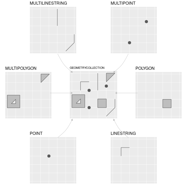
## Seven common Simple Feature (SF) geometry types
| type | description |
| ---- | ----------- |
| `POINT` | a single point |
| `LINESTRING` | sequence of points connected by lines |
| `POLYGON` | sequence of points form a closed ring |
| `MULTIPOINT` | set of points |
| `MULTILINESTRING` | set of linestrings |
| `MULTIPOLYGON` | set of polygons |
| `GEOMETRYCOLLECTION` | set of geometries |
Some formats only include these (e.g. [GeoJSON](https://tools.ietf.org/html/rfc7946))
## Uncommon Geometry Types
10 more geometries 10 are rare:
* `CIRCULARSTRING`
* `COMPOUNDCURVE`
* `CURVEPOLYGON`
* `MULTICURVE`
* `MULTISURFACE`
* `CURVE`
* `SURFACE`
* `POLYHEDRALSURFACE`
* `TIN`
* `TRIANGLE`
---
## Coordinate reference system
SFs can only be placed on the Earth's surface when their coordinate
reference system (CRS) is known; this may be an elipsoidal CRS such as WGS84, a projected, two-dimensional (Cartesian) CRS such as a UTM zone or Web Mercator, or a CRS
in three-dimensions or [including time](http://www.faculty.jacobs-university.de/pbaumann/iu-bremen.de_pbaumann/Papers/acmgis-2012_crs-nts.pdf). Similarly, M-coordinates need an attribute reference
system, e.g. a [measurement unit](https://CRAN.R-project.org/package=units).
---
There are currently two main approaches in R to handle geographic vector data.
---
## `sp` package
First package for spatial data: [`sp`](https://cran.r-project.org/package=sp). Provides classes and methods to create _points_, _lines_, _polygons_, and _grids_ and to operate on them.
~350 of the spatial analysis packages use `sp` data types, so it is important to know how to convert **sp** to and from **sf** objects.
## `sf` package
[`sf`](https://cran.r-project.org/package=sf) implements a formal standard called ["Simple Features"](https://en.wikipedia.org/wiki/Simple_Features) that specifies a storage and access model of spatial geometries (point, line, polygon).
A feature geometry is called simple when it consists of points connected by straight line pieces, and does not intersect itself.
This standard has been adopted widely, not only by spatial databases such as PostGIS, but also more recent standards such as GeoJSON.
## How simple features in R are organized
All spatial functions and methods in `sf` prefixed by `st_` (refering to _spatial and temporal_)
Simple features are implemented as R native data, using simple data structures (S3 classes, lists,
matrix, vector).
---
Stored as `data.frame` objects (or very similar `tbl_df`) with _feature geometries in
a `data.frame` column_.
Since geometries are not single-valued,
they are put in a list-column, a list of length equal to the number
of records in the `data.frame`, with each list element holding the simple
feature geometry of that feature.
## Components
* `sf`, the table (`data.frame`) with feature attributes and feature geometries, which contains
* `sfc`, the list-column with the geometries for each feature (record), which is composed of
* `sfg`, the feature geometry of an individual simple feature.
---
If you work with PostGis or GeoJSON you may have come across the [WKT (well-known text)](https://en.wikipedia.org/wiki/Well-known_text) format, for example like these:
POINT (30 10)
LINESTRING (30 10, 10 30, 40 40)
POLYGON ((30 10, 40 40, 20 40, 10 20, 30 10))
`sf` implements this standard natively in R. Data are structured and conceptualized very differently from the `sp` approach.
---
## I. Create geometric objects (topology)
Geometric objects (simple features) can be created from a numeric vector, matrix or a list with the coordinates. They are called `sfg` objects for Simple Feature Geometry.
Create a LINESTRING `sfg` object:
```{r}
xy=matrix(runif(6), ncol=2)
xy
lnstr_sfg <- st_linestring(xy)
class(lnstr_sfg)
lnstr_sfg
```
---
## II. Combine all individual single feature objects for the special column.
Create a `sfc` (Simple Feature Collection) object of individual features:
```{r}
lnstr_sfc <- st_sfc(lnstr_sfg) # just one feature here
class(lnstr_sfc)
lnstr_sfc
```
The `sfc` object also holds the bounding box and the projection information.
## III. Add attributes.
Add attributes (in a `data.frame`) to the `sfc` object to make a `sf` (Simple Features) object:
```{r}
dfr=data.frame(type="random")
lnstr_sf <- st_sf(dfr , lnstr_sfc)
class(lnstr_sf)
lnstr_sf
```
---
```{r, echo=F}
knitr::kable(lnstr_sf)
```
---
## sf Highlights
* provides **fast** I/O, particularly relevant for large files
* directly reads from and writes to spatial **databases** such as PostGIS
* compatibile with the *tidyverse*
* recent `ggplot` release can read and plot the `sf` format without conversion
---
`sp` and `sf` are _not_ only formats for spatial objects. Other spatial packages may use their own class definitions for spatial data (for example `spatstat`). Usually you can find functions that convert `sp` and increasingly `sf` objects to and from these formats.
## Converting formats
```{r}
data(world) #load 'world' data from spData package
world_sp = as(world, "Spatial") # convert from sf to sp
world_sf = st_as_sf(world_sp) #convert from sp to sf
str(world_sp)
```
---
```{r}
str(world)
```
---
- The structures in the **sp** packages are more complicated - `str(world_sf)` vs `str(world_sp)`
- Moreover, many of the **sp** functions are not "pipeable" (it's hard to combine them with the **tidyverse**)
```{r, eval = F}
world_sp %>%
filter(name_long == "Papua New Guinea")
```
`Error in UseMethod("filter_") : no applicable method for 'filter_' `
`applied to an object of class "c('SpatialPolygonsDataFrame', 'SpatialPolygons',`
`'Spatial', 'SpatialPolygonsNULL', 'SpatialVector')"`
```{r}
world %>%
filter(name_long == "Papua New Guinea")
```
---
## Reading and writing spatial data
```{r}
vector_filepath = system.file("shapes/world.gpkg", package = "spData")
vector_filepath
world = st_read(vector_filepath)
```
Counterpart to `st_read()` is the `st_write` function, e.g. `st_write(world, 'data/new_world.gpkg')`. A full list of supported formats could be found using `sf::st_drivers()`.
---
## Structure of the sf objects
```{r, eval = FALSE}
world
```
```{r, echo = FALSE}
print(world, n=3)
```
```{r}
class(world)
```
---
## Structure of the sf objects
```{r, eval=FALSE}
world$name_long
```
```{r, echo=FALSE}
world$name_long[1:3]
```
```{r, eval=FALSE}
world$geom
```
```{r, echo=FALSE}
print(world$geom, n = 3)
```
## Non-spatial operations on sf objects
> Which countries have the highest population density?
```{r}
print(world, n=3)
print(worldbank_df, n=3)
```
---
```{r, warning=FALSE}
pop_den <-
world %>%
left_join(worldbank_df, by = "iso_a2") %>%
mutate(pop_density = pop/area_km2) %>%
dplyr::select(name_long, pop_density) %>%
arrange(desc(pop_density))
```
```{r echo=F}
pop_den%>%
slice(1:5)%>%
st_set_geometry(NULL)%>%
knitr::kable()
```
---
```{r}
ggplot(pop_den)+
geom_sf(aes(fill=pop_density,geometry=geom))+
scale_fill_viridis_c()
```
## Non-spatial operations
```{r}
world_cont = world %>%
group_by(continent) %>%
summarize(pop_sum = sum(pop, na.rm = TRUE))%>%
arrange(desc(pop_sum))
```
```{r, echo=FALSE}
print(world_cont, n = 3)
```
---
The `st_set_geometry` function can be used to remove the geometry column:
```{r}
world_df =st_set_geometry(world_cont, NULL)
class(world_df)
```
---
## Spatial operations
It's a big topic which includes:
- Spatial subsetting
- Spatial joining/aggregation
- Topological relations
- Distances
- Spatial geometry modification
- Raster operations (map algebra)
See [Chapter 4](http://robinlovelace.net/geocompr/spatial-data-operations.html#spatial-operations-on-raster-data) of *Geocomputation with R*
## CRS
Transform (warp) to a different projection:
```{r}
na_2163 = world %>%
filter(continent == "North America") %>%
st_transform(2163) #US National Atlas Equal Area
st_crs(na_2163)
```
---
## Compare projections
```{r, message=F}
library(gridExtra) # for combining ggplots
na = world %>% filter(continent == "North America")
p1=na_2163 %>% ggplot()+geom_sf(aes(geometry=geom))
p2=na %>% ggplot()+geom_sf(aes(geometry=geom))
grid.arrange(p1,p2,nrow=1)
```
For more on `grid.arrange`, see [here](https://cran.r-project.org/web/packages/egg/vignettes/Ecosystem.html).
---
## Spatial operations
```{r, warning = FALSE, message = FALSE, fig.height = 4}
canada = na_2163 %>%
filter(name_long=="Canada")
canada_buffer=canada%>%
st_buffer(500000)
ggplot()+
geom_sf(data=canada,aes(geometry=geom))+
geom_sf(data=canada_buffer,col="red",fill=NA)
```
# Visualization
## Basic maps
- Basic maps of `sf` objects can be quickly created using the `plot()` function:
```{r}
plot(world[0])
```
---
```{r}
plot(world["pop"])
```
## ggplot and geom_sf()
```{r}
ggplot(world)+
geom_sf(aes(geometry=geom,fill=lifeExp))+
scale_fill_viridis_c()
```
All the nice ggplot features are available
## leaflet: javascript library for interactive maps
```{r, message=F}
library(leaflet)
library(widgetframe)
```
[Leaflet](https://leafletjs.com/) leading open-source JavaScript library for mobile-friendly interactive maps. Weighing just about 38 KB of JS, it has all the mapping features most developers ever need.
## Construct the leaflet map
```{r}
l=leaflet(world) %>%
addTiles() %>%
addPolygons(color = "#444444", weight = 1, fillOpacity = 0.5,
fillColor = ~colorQuantile("YlOrRd", lifeExp)(lifeExp),
popup = paste("Life Expectancy =", round(world$lifeExp, 2)))
```
```{r, echo=F, eval=F,message=F}
f <-"presentations/world_leaflet.html"
saveWidget(l,file.path(normalizePath(dirname(f)),basename(f)),
libdir="externals",
selfcontained = T)
```
<iframe id="test" style=" height:400px; width:100%;" scrolling="no" frameborder="0" src="world_leaflet.html"></iframe>
Page hosted on Github for free (except the domain name)...
---
## Raster data in the tidyverse
Raster data is not yet closely connected to the **tidyverse**, however:
- Some functions from `raster` work well in `pipes`
- Convert vector data to `Spatial*` form using `as(my_vector, "Spatial")` for raster-vector interactions
- Some early efforts to bring raster data into the **tidyverse**, including [tabularaster](https://github.com/hypertidy/tabularaster), [sfraster](https://github.com/mdsumner/sfraster), [fasterize](https://github.com/ecohealthalliance/fasterize), and [stars](https://github.com/r-spatial/stars) (multidimensional, large datasets).
---
## Sources
- Slides adapted from:
- "Robin Lovelace and Jakub Nowosad" draft book [_Geocomputation with R_ (to be published in 2018)](http://robinlovelace.net/geocompr/). Source code at https://github.com/robinlovelace/geocompr.
- [Claudia Engel's spatial analysis workshop](https://github.com/cengel/rspatial/blob/master/2_spDataTypes.Rmd)