Bayesian optimization

Bayesian optimization is a sequential model-based strategy for global optimization of black-box objective functions whose evaluations are costly. It is commonly used when a single observation requires an experiment, engineering computation, numerical simulation, or machine-learning run, and when derivatives are unavailable or unreliable. The objective need not have a closed-form expression.

The method constructs a probabilistic model of the unknown function, often a Gaussian process (GP), and uses the resulting predictive distribution to choose the next evaluation point. This choice is made by optimizing a sampling criterion, also called an acquisition function.

Common applications include hyperparameter optimization in machine learning, where each trial may require training and validating a model, and engineering design problems driven by expensive numerical simulations.

History

Early Bayesian approaches to global optimization include work by Harold J. Kushner on locating extrema of noisy functions and work by Jonas Mockus on Bayesian methods for seeking extrema.

Expected improvement is a prominent sampling criterion in this line of work. In 1998, Donald R. Jones, Matthias Schonlau, and William J. Welch introduced the efficient global optimization (EGO) algorithm, which used a kriging or Gaussian-process model with expected improvement for expensive black-box functions.

Later work extended Bayesian optimization to noisy observations, constraints, batch and parallel evaluations, multiple objectives, and mixed or high-dimensional search spaces.

Problem setting

In a standard single-objective setting, Bayesian optimization seeks a point

$x^{\star }\in \operatorname {arg\,min} _{x\in {\mathcal {X}}}f(x)$

where ${\mathcal {X}}$ is a search space and $f$ is an unknown objective function. A maximization problem can be written in the same form by minimizing $-f$. Although the search space may in principle be continuous, discrete, categorical, or mixed, the standard formulation is most directly applicable to continuous, low- to moderate-dimensional domains. Later methods attempt to relax these restrictions by addressing mixed variables, high-dimensional spaces, constraints, parallel evaluations, and multiple objectives.

A useful distinction is between noiseless and noisy optimization. Many real applications also involve constraints, parallel evaluations, or multiple objectives. These variants change how the probabilistic model, incumbent solution, and sampling criterion are defined.

Basic method

Bayesian optimization of a one-dimensional function. A probabilistic model is updated after observations, and sampling criteria guide the selection of future evaluation points.

A typical Bayesian optimization procedure builds a sequence of evaluation points. Starting from an initial design $X_{0}$, the algorithm produces additional evaluation points $x_{1},x_{2},\ldots$. After $n$ sequential evaluations, $X_{n}=X_{0}\cup \{x_{1},\ldots ,x_{n}\}$ denotes the evaluated points and ${\mathcal {D}}_{n}$ denotes the corresponding observations. The next point $x_{n+1}$, or a batch of points, is selected by optimizing a sampling criterion computed from the current probabilistic model.

The procedure has the following form:

1. Choose an initial design $X_{0}$, often by a space-filling design or random sampling.
2. Evaluate the objective function, and any constraints if present, at the initial design points.
3. Construct or update a probabilistic model using the observed data ${\mathcal {D}}_{n}$.
4. Define a sampling criterion, also called an acquisition function or infill criterion, from the probabilistic model.
5. Optimize the sampling criterion to select $x_{n+1}$, or a batch of points, for evaluation.
6. Evaluate the selected point or points and update the data set.
7. Repeat until an evaluation budget, convergence criterion, or stopping rule is reached.

The Bayesian strategy treats the unknown objective as a random function and places a prior over it. The prior captures assumptions about the behavior of the function. After observations are collected, the prior is updated to form a posterior distribution over the objective function. The posterior distribution is then used to construct the sampling criterion that determines the next query point.

Probabilistic models

Bayesian optimization requires a probabilistic model of the unknown objective function and, when present, of unknown constraints. Given the evaluations observed so far, the model gives a predictive distribution for unevaluated points in the search space. Sampling criteria are defined from this predictive distribution, so the model provides both predicted objective values and uncertainty estimates. Such probabilistic models are often called surrogate models or metamodels because they are used in place of direct evaluations of the expensive objective when choosing candidate points.

Gaussian process regression is the standard probabilistic model in classical presentations of Bayesian optimization and remains common in applications. A Gaussian process prior defines a distribution over functions. After observations are collected, the posterior predictive mean and variance are used by sampling criteria such as expected improvement, probability of improvement, and upper confidence bound criteria. Other probabilistic models can be used when the search space, dimensionality, or data size favors another representation.

Variants and problem classes

Bayesian optimization is often described through a noiseless, single-objective problem, but the same model-based loop is adapted to several related settings.

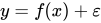
In noisy Bayesian optimization, evaluations return observations such as $y=f(x)+\varepsilon$ instead of exact values of the latent objective. The probabilistic model can represent both uncertainty about $f$ and observation noise. Classical expected improvement over the best observed value is a noiseless criterion. In noisy settings, recommendation rules and sampling criteria may be defined for the latent objective, for future noisy observations, or for the value of information. Examples include knowledge-gradient and information-theoretic criteria.

In constrained Bayesian optimization, the objective is optimized subject to feasibility constraints. If the constraints are also unknown black-box functions, separate probabilistic models can be constructed for the objective and constraints, and the sampling criterion can combine predicted improvement with the probability of feasibility.

In batch or parallel Bayesian optimization, the method proposes several candidate points before the corresponding observations are available. Batch methods are useful when experiments, simulations, or machine-learning jobs can be executed concurrently. They may optimize a joint sampling criterion or choose points sequentially while accounting for pending evaluations.

In multi-objective Bayesian optimization, several objective functions are optimized at once and the result is typically an approximation to a Pareto front. Methods include scalarization approaches such as ParEGO, which reduce the problem to a sequence of single-objective subproblems, and indicator-based approaches using criteria such as expected hypervolume improvement. Constrained multi-objective Bayesian optimization combines these extensions by modeling objectives and constraints and using sampling criteria based on extended domination rules and expected hypervolume improvement.

Sampling criteria

A sampling criterion, also called an acquisition function in the machine-learning literature or an infill criterion in surrogate-based optimization, scores candidate points using the current predictive distribution. It is usually inexpensive to evaluate and is optimized instead of the expensive objective function. Sampling criteria express the exploration-exploitation tradeoff by assigning high values to points with a low predicted objective value, high uncertainty, or both. A seminal example in the noiseless setting is expected improvement, which scores a candidate point by the posterior expected gain over the best value observed so far. Other criteria include probability of improvement, upper- or lower-confidence-bound criteria such as GP-UCB, Thompson sampling, knowledge-gradient criteria, information-theoretic criteria including the IAGO minimizer-entropy criterion, entropy search, and predictive entropy search, and portfolios or hybrids of several criteria.

Expected improvement

Expected improvement (EI) was used in the efficient global optimization (EGO) algorithm and remains a standard reference criterion for noiseless Bayesian optimization. In the noiseless minimization setting, let $f_{\min }$ be the best objective value observed so far and let ${\mathcal {D}}$ denote the data. The expected improvement at a candidate point $x$ is

$\operatorname {EI} (x)=\mathbb {E} [\max(f_{\min }-f(x),0)\mid {\mathcal {D}}]$.

When the model predictive distribution at $x$ is Gaussian, $f(x)\mid {\mathcal {D}}\sim {\mathcal {N}}(\mu (x),\sigma ^{2}(x))$, and $\sigma (x)>0$, EI has the closed form

$\operatorname {EI} (x)=(f_{\min }-\mu (x))\Phi (z)+\sigma (x)\phi (z),\quad z={\frac {f_{\min }-\mu (x)}{\sigma (x)}}$,

where $\Phi$ and $\phi$ are the cumulative distribution function and probability density function of the standard normal distribution. EI is therefore large when the model predicts a low objective value, when uncertainty is high, or both.

Solution methods

The sampling criterion is usually cheap to evaluate relative to the objective, but optimizing it can still be a nonconvex auxiliary problem. Its optimum is often sought by discretization, multi-start local optimization, or deterministic numerical methods such as Newton's method and quasi-Newton methods like the Broyden–Fletcher–Goldfarb–Shanno algorithm. Stochastic methods are also used for this auxiliary search, especially for multimodal or mixed-variable criteria. Examples include genetic algorithms and other evolutionary algorithms, as well as sequential Monte Carlo methods.

Related methods

Several derivative-free optimization methods use probability distributions without modeling the unknown objective function itself. Estimation of distribution algorithms build and sample explicit probabilistic models of selected candidate solutions. The cross-entropy method and CMA-ES also update parametric sampling distributions, with CMA-ES adapting the mean, step size, and covariance matrix of a multivariate normal distribution. These methods use objective values to update a distribution over candidate points. In Bayesian optimization, the probabilistic model instead represents the objective or constraints, and the next point is chosen by optimizing a criterion derived from that model.

Gaussian-process sequential design is also used in reliability analysis to estimate a probability of failure. For a limit-state function $f$, random input $X$, and threshold $t$, the target may be $\mathbb {P} (f(X)\leq t)$, or more generally the measure of an excursion set. Stepwise uncertainty reduction strategies choose evaluations to reduce uncertainty about this probability, rather than to locate the minimizer or maximizer of $f$.

Bayesian optimization is also related to multi-armed bandit problems. Both study sequential decisions that trade off exploration and exploitation, and criteria such as upper confidence bounds and Thompson sampling appear in both settings. A common distinction is that bandit algorithms are often formulated to control cumulative regret over a sequence of actions, while Bayesian optimization often emphasizes finding a good optimizer of an expensive function after a small evaluation budget.

Applications

Bayesian optimization is used in applications where objective evaluations are costly. Examples discussed in surveys and textbooks include hyperparameter optimization and algorithm configuration, engineering design and simulation-based optimization, robotics, sensor networks, and experimental design in the physical sciences.

See also

• Multi-armed bandit
• Kriging
• Thompson sampling
• Global optimization
• Bayesian experimental design
• Probabilistic numerics
• Pareto optimum
• Active learning (machine learning)
• Multi-objective optimization